Roughness, Interlayers, and a Dirty Surface

The models of Chapters 5 and 6 had sharp boundaries and identical periods. Real samples don’t. Their boundaries have a width. Two materials can mix and form a thin layer of their own. Every surface in air carries a light film of hydrocarbons. And the period can change from the bottom of the stack to the top. Each of these leaves its own mark on the curve. This chapter builds on Chapter 6: The higher orders carry the fine details.

A boundary with a width

A real boundary is never a perfect step. The surface can be rough. The two materials can mix near the boundary. Even the atoms have a size. So the change from one material to the next is spread over a width. X-Ray Calc calls that width the roughness σ. As in Chapter 5: What roughness does to the fringes, the σ of a layer belongs to its upper interface.

Figure 7-1: Three boundaries between a light material (top) and a heavy one (bottom). (a) Sharp: the density jumps at one depth. (b) Rough: the boundary is sharp, but its height changes from place to place. (c) Intermixed: the two materials blend over a range of depths. When (b) and (c) have the same average density at each depth, their reflectivity curves are the same.

A wide boundary reflects less than a sharp one. The parts of the wave reflected at different depths within the boundary are out of step, so they partly cancel. X-Ray Calc treats every boundary as Gaussian. It multiplies the reflection of each interface by

\exp\!\left(-\tfrac{1}{2}\,q_0\,q'\,\sigma^2\right)

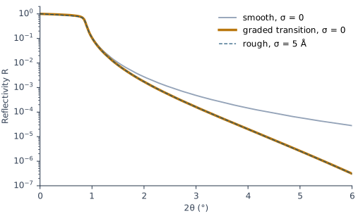
Here $q_0 = 4\pi\sin\theta/\lambda$ is the wave-vector transfer in vacuum, and $q'$ is the one refracted across the interface. This form is the Névot–Croce factor. Well above the critical angle $q' \approx q_0$ . The reflectivity of the boundary then falls by about $\exp(-q^2\sigma^2)$ . The loss grows fast with angle. For a Mo surface with σ = 5 Å, X-Ray Calc gives 0.63 of the smooth reflectivity at θ = 1°, 0.14 at θ = 2° and 0.011 at θ = 3° (Figure 7-2). So roughness lowers the high Bragg orders first.

Going Deeper: Debye–Waller against Névot–Croce

The simplest treatment of a Gaussian boundary uses the wave-vector transfer in vacuum on both sides. It reduces the reflected intensity by $\exp(-q^2\sigma^2)$ , the Debye–Waller factor. Near the critical angle this overestimates the loss, because the wave inside the material travels at a much smaller angle. Its $q$ is much smaller than in vacuum. Replacing $q^2$ by the product of the two sides’ values, $q_1 q_2$ , gives a very good approximation to the exact result (Spiller, Eqs. 7.17–7.18). This is the Névot–Croce factor. X-Ray Calc uses it on every interface, for s- and p-polarization alike.

The difference shows at small angles. For the rough Mo surface of Figure 7-2, at θ = 0.5°, X-Ray Calc keeps 0.94 of the smooth reflectivity. The Debye–Waller factor would keep only 0.88. At θ = 3° both give 0.011.

Roughness and intermixing look the same

A rough boundary and an intermixed one are different things. Figure 7-1 shows both. The specular reflectivity can’t tell them apart. It sees only the density at each depth, averaged over the area the beam lights. A rough boundary and a blended one with the same average profile give the same curve.

Figure 7-2 shows this for a Mo surface. One curve has σ = 5 Å. The other has σ = 0, but it is built from 80 slices of Mo 0.5 Å thick. Their density rises smoothly, most of it within 20 Å, with the same average profile as the rough surface. Above the critical edge the two curves differ by at most 0.5 %. Over the same range, the roughness itself lowers the reflectivity by up to a factor of 90.

Calculated reflectivity of a molybdenum surface: smooth, rough with sigma 5 angstrom, and a graded transition built from thin slices. The rough and graded curves lie on top of each other, well below the smooth one — **Figure 7-2:** A rough surface and a graded one give the same curve. Bare Mo at λ = 1.5406 Å. Gray: smooth. Blue dashes: σ = 5 Å. Orange: σ = 0, with 80 slices of Mo 0.5 Å thick whose density rises from almost zero to bulk over the same average profile. Above the critical edge the two lower curves differ by at most 0.5 %. Calculated by X-Ray Calc 3.9.4.1250 with no resolution blur.

Interlayers: when the two interfaces of a period differ

Two materials often react or mix where they meet. The mixed zone can be thick enough to act as a layer of its own, an interlayer. In X-Ray Calc an interlayer is one more layer in the period, with a compound material such as CoC or MoSi2.

The two interfaces of a period need not be alike. A heavy material deposited on a light, amorphous one grows differently from a light material deposited on a heavy one. The fitting procedure notes that the resulting interlayers can differ in width (§10.9). The X-Ray Calc Help shows this for Mo/Si mirrors, which have asymmetric intermixed zones.

An interlayer changes the curve strongly. Which side it sits on changes it much less. Figure 7-3 shows a Co/C stack with the period of Chapter 6, 50 Å, with and without an 8 Å CoC interlayer. With the interlayer, the 2nd order falls to 0.47 of its height, and the 4th to 0.09. Moving the same interlayer to the other interface changes the order heights by at most 12 %. The difference shows mostly in the fringes between the orders.

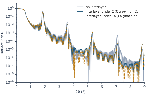
Three calculated Co/C multilayer curves: without an interlayer, with an interlayer under the carbon layer, and with it under the cobalt layer. The two interlayer curves have almost the same Bragg orders and differ between them — **Figure 7-3:** An interlayer and its side. Co/C on Si, 20 periods, D = 50 Å, σ = 3 Å everywhere, at λ = 1.5406 Å. Gray: 31.2 Å C over 18.8 Å Co. Blue and orange: 4 Å of each layer replaced by 8 Å of CoC, under the C layer (blue) or under the Co layer (orange). The interlayer changes the order heights strongly. Its side changes them by at most 12 %. Calculated by X-Ray Calc 3.9.4.1250 with no resolution blur.

So the curve fixes the amount of mixing better than its side. The top of the stack and the roughness also show in those fringes. So the fringes alone are a weak guide to the side. The fitting procedure reports a case: two independent fits of one curve “agreed on the total metal in a period to within a few tenths of an angstrom while placing the thick interlayer on opposite sides of the metal layer” (§10.8).

The same holds for the two roughnesses of a period. On the measured Co/C curve CoC4, one fit gave σ = 2.64 Å for C and 4.33 Å for Co. The expert’s fit gave the opposite pair, 5.58 Å and 2.46 Å. A third fit found 5.70 Å and 2.75 Å. All three put the same peaks at the same period. Only the fringes between the orders differ. The random start of the fit decided which pair it found.

The dirty surface: a contamination layer

Every surface that has been in air carries a thin layer of hydrocarbons. It is light and thin, but the curve sees it. The fitting procedure adds it to the starting model because “without it the fringe fields between the orders do not fit” (§2.3).

On the author’s instrument the starting values are 15 Å of C with σ = 3 Å and ρ = 0.9 g/cm³. The fit limits are 5–40 Å, 1–10 Å and 0.6–1.4 g/cm³. These are one laboratory’s values, an example rather than a rule. The layer is its own stack with N = 1, above the periodic stack.

Figure 7-4 shows the effect on the measured Co/C curve CoC4. The fit without the layer puts the level between the 2nd and 3rd orders too high. In the band 2θ = 3.11–4.46° its mean residual is +0.133 in log₁₀, a factor of 1.36. With the layer, the mean residual falls to −0.064, and χ² falls from 7.94 to 6.09. The fitted layer was 12.6 Å thick, with ρ = 0.68 g/cm³. Nothing in the period stack moved: the period stayed at 54.70–54.72 Å.

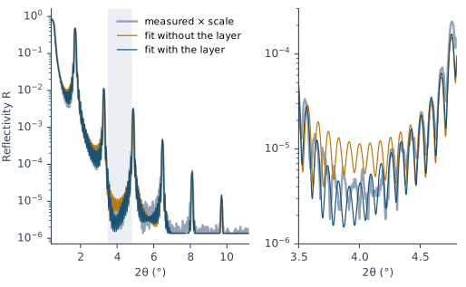
A measured Co/C multilayer curve with two fits. On the left the whole curve, on the right the region between the second and third Bragg orders, where the fit without a surface layer lies too high and the fit with it follows the data — **Figure 7-4:** A contamination layer on a measured curve. Gray: the Co/C multilayer CoC4, measured with Cu Kα and multiplied by the fit's scale. Orange: the fit without a surface layer (χ² = 7.94). Blue: the fit with a carbon layer on top (χ² = 6.09). Left: the whole fitted range. The shaded band is magnified on the right. There the fit without the layer runs above the data between the 2nd and 3rd orders. Data: the fitting procedure's data deposit.

The single carbon film of Chapter 5 told the same story. Its refit put 300.5 Å of carbon under a contamination layer 13 Å thick. The fringes had measured the two together (Chapter 5: Reading a thickness from the fringes).

A stack that drifts

A deposition rate can change during a long run. The layers deposited early then differ in thickness from those deposited late. The period changes with depth. This book calls an accidental change of this kind a drift. A change made on purpose is a graded stack (Chapter 22: Graded on purpose).

A drift spreads the Bragg orders. Each period puts its orders at slightly different angles. The spread grows with the order number, as Chapter 6: The higher orders carry the fine details explained. Figure 7-5 shows the drifting stack of the Chapter 3 demo, a Mo/Si stack whose period runs from 40.00 Å at the top to 43.60 Å and back to 41.96 Å. It is compared with a uniform stack of the same mean period, 42.30 Å. The 1st order keeps 0.88 of its height. The 2nd to 5th orders keep only 0.25 to 0.49. The 2nd and 4th orders become about three times as wide.

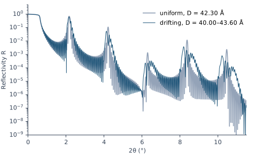
Calculated curves of a uniform Mo/Si multilayer and of one whose period drifts through the stack. The first Bragg order is almost the same. The higher orders of the drifting stack are lower and wider — **Figure 7-5:** A drift lowers and widens the high orders. Mo/Si on Si, 30 periods of Si over 15 Å Mo, all smooth, at λ = 1.5406 Å. Gray: every Si layer 27.30 Å (D = 42.30 Å). Blue: the Si thickness of the Chapter 3 demo, which gives periods from 40.00 Å at the top to 43.60 Å and 41.96 Å next to the substrate, with the same mean. Calculated by X-Ray Calc 3.9.4.1250 with no resolution blur, one stack per period.

A fit with one period for the whole stack can’t follow this. The fitting procedure describes the sign: the fit reproduces the low orders, but shows “the calculated Bragg maxima standing clearly above the measured ones, and further above them the higher the order” (§9.3). X-Ray Calc describes a drift with a profile. The value of a layer parameter then changes from period to period as a polynomial. Polynomial mode fits it, as the demo fit of Chapter 3: What the fit found did.

What this means when you fit

Don’t let σ stand in for a missing layer. A roughness or a density can often be pushed to a value that hides a feature the model lacks. The fitting procedure is clear about this: “A model that is too simple is fixed by adding what is missing (a light surface layer of contamination, an interlayer at an interface, a drift through the stack), not by pushing a parameter that stands in for it” (§10.13). A σ that sits on its fit limit is a warning sign.

Add the contamination layer when the edge or the level between the orders misses. That is the rule of the author’s preset. Chapter 12: The top of the stack puts the layer into the model.

Report σ as a width. It includes roughness and intermixing. Don’t claim which interface of a period is the rougher one, or on which side an interlayer sits, unless repeated fits agree (Chapter 18: Asymmetric interlayers; Chapter 23: Writing the numbers).

Watch the high orders for a drift. If a one-period fit matches the low orders and overshoots the high ones, try Polynomial mode (Chapter 17: What a drift does to the orders).

Sources

Fitting procedure (Penkov, Peng & Fu 2026): §2.3, the light surface layer “stands for the hydrocarbon contamination every surface carries in air; without it the fringe fields between the orders do not fit”; §3.3 rule 1, the level between the peaks set by the ends of the stack; §9.3, the drift pattern across the orders; §10.8–10.9, the interlayer total fixed but not its side, and asymmetric growth; §10.13, a model too simple is fixed by adding what is missing; §10.14, the two roughnesses of a two-material period and the seed.
The author’s instrument preset (skill-v5\presets\csmic-empyrean.json, surface.contamination_layer): C, 15 Å, σ 3 Å, ρ 0.9 g/cm³; limits 5–40 Å, 1–10 Å, 0.6–1.4 g/cm³; included when the edge or the fringe field misses without it.
Methods paper, Supplementary S4.6 (si\S4-results-in-full.md): the CoC4 roughness pairs (2.64/4.33 Å, the expert’s 5.58/2.46 Å, a test session’s 5.70/2.75 Å); χ² 7.94 → 6.09 with the surface layer; the band residual +0.133 → −0.064; “Nothing in the period stack moved”. The layer thickness, density and periods are from the paper’s surface-layer figure (deposit figures/fig7-surface-layer.png).
The measured curve CoC4 (record P2-04, a Co/C multilayer of 20 periods on glass) and the two fits of Figure 7-4 (jobs fit-20260919-061017-879e and -4587) are from the fitting procedure’s data deposit (CC BY 4.0), jobs/figure-data/fig7-CoC4-* and jobs/seed-and-surface-study/. They are read in place and not copied into the book. The χ² values and band residuals are read from the jobs’ report.json.
Spiller, E. (1994). Soft X-ray Optics. SPIE. A boundary of finite width from roughness, intermixing and atomic size, and its Gaussian description (p. 110, Eqs. 7.15–7.16); the Debye–Waller factor (p. 111, Eq. 7.17); its overestimate near the critical angle, and the geometric mean q₁q₂ as a very good approximation to the rigorous theory (p. 112, Eq. 7.18, Fig. 7.3); boundaries sharp to about 1/10 of the period (p. 112); for the specular reflectivity a gradual, homogeneous transition has the same effect as a rough boundary with the same profile (pp. 113–114); roughness separated from intermixing only by other methods such as scattering and microscopy (§10.4–10.5).
Névot, L. & Croce, P. (1980). Caractérisation des surfaces par réflexion rasante de rayons X. Application à l’étude du polissage de quelques verres silicates. Revue de Physique Appliquée 15, 761–779. doi:10.1051/rphysap:01980001503076100. The original paper of the roughness factor. The chapter’s account of the factor follows Spiller.
X-Ray Calc Help: Calculation → Algorithm (Gaussian roughness, the factor exp(−q₀q′σ²/2), the same for s and p); Models → Layers, Stacks (Periods) (σ of the upper interface; Structure > Add Stack and the Stack Properties dialog); Profiles (function profiles by period number from the surface); Examples → Periodic X-Ray Mirrors (asymmetric intermixed zones in Mo/Si).
The X-Ray Calc 3 source: the roughness factor, rfError, the only one the program uses (Shared\Math\unit_calc.pas, Roughness), applied to each interface with the σ of the layer below it (unit_calc.pas, the call with AModel.s[i + 1]). Before 3.9.4.1050 the exponent used 0.50299 in place of ½. Later builds use exactly ½ (release 3.9.4.1250, unit_calc.pas:463). The Help’s note on the change (Calculation → Algorithm) dates it to 3.9.4. The first build with ½ is 3.9.4.1050, and the book follows the code.
Calculated for this chapter (2026-09-24, rerun 2026-09-25) with the X-Ray Calc 3.9.4.1250 engine at λ = 1.5406 Å, with no resolution blur, s-polarization and the reflectivity floor lowered to 10⁻¹²: the Mo surfaces of Figure 7-2, the Co/C stacks of Figure 7-3 (the CoC table at its bulk density), and the Mo/Si stacks of Figure 7-5 (the Chapter 3 demo’s Si profile, one stack per period). scripts/figures/ch7_engine_data.py runs the calculations and keeps the curves in figures-src/ch7/. scripts/figures/fig_7_figures.py draws Figures 7-2 to 7-5 and computes every ratio, order height and width quoted in the text.

Cross-references: Chapter 3: What the fit found; Chapter 5: What roughness does to the fringes; Chapter 6: The higher orders carry the fine details; Chapter 8; Chapter 12; Chapter 13; Chapter 17: What a drift does to the orders; Chapter 18: Which interface is rougher?; Chapter 22: Graded on purpose; Chapter 23: Writing the numbers; Chapter 26: The shape of an interface; Appendix A: Notation and Units; Appendix D: Glossary.