Every fit returns a density for every layer, and the number looks like a material property. This chapter shows why it isn’t one, what a density can still tell you, and how to report it. It uses the fits of the two measured Co/C curves made in Chapters 14 to 19, and the fitting procedure’s tests on curves calculated from a known structure. It needs no new fit.
A free parameter, not a result
The fitting procedure is short on this point: “A fitted density is a free parameter, never a result. Do not report it as a material property, do not build a design, a rule or a deposition time on it, and do not spend fits determining it.” (§11.1) The author said it more briefly when the procedure was written down: “We don’t really care about density.”
The reason is in what the curve sees. X-Ray Calc takes the optical constants of each material from its Henke table and changes them only through the density. δ grows in proportion to ρ (Chapter 4: What this means when you fit). So the curve fixes the δ of each layer, and the fit turns it into a ρ. Several other things change the curve in a similar way:
- The scale. The density of Co raises every order and the edge together, as a higher scale does (Chapter 13: The variants and what they move). With the scale held at a wrong anchor, the CoC4 fit put Co 0.49 g/cm³ higher (Chapter 14: Table 14-2).
- A missing layer. Without the contamination layer, the C of the period took over its work, and its density fell from 2.00 to 1.77 g/cm³ (Chapter 19: Table 19-3).
- Mixing at the interfaces. A metal layer with a mixed zone on each side holds less metal per angstrom. A single layer of lower density can look the same to the curve.
So a density takes up whatever the model and the data conditioning leave over. You can’t read it as the density of the material.
The runs agree, the models don’t
Chapter 16 reports a spread over five runs beside every fitted value. For a density that spread is small, and it misleads. Figure 20-1 and Table 20-1 give the Co density of CoC4 and CoC5 under every model this book fitted.
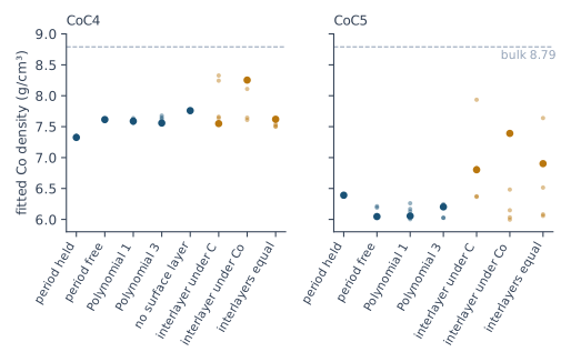
Table 20-1: The fitted densities of the run with the lowest χ², with the sample standard deviation over five runs in brackets, in g/cm³. The bulk densities of the tables are 8.79 for Co and 2.266 for C. Fitted by X-Ray Calc 3.9.4.1250 and 3.9.4.1270.
| Model | CoC4: Co | CoC4: C | CoC5: Co | CoC5: C |
|---|---|---|---|---|
| Periodic, period held | 7.33 (0.01) | 2.00 (0.02) | 6.39 (0.01) | 2.23 (0.00) |
| Periodic, period free | 7.61 (0.01) | 2.00 (0.00) | 6.05 (0.09) | 2.08 (0.03) |
| Polynomial, order 1 | 7.59 (0.03) | 2.04 (0.02) | 6.06 (0.10) | 2.05 (0.05) |
| Polynomial, order 3 | 7.56 (0.05) | 1.96 (0.04) | 6.20 (0.11) | 2.17 (0.05) |
| Period free, no surface layer | 7.76 (0.01) | 1.77 (0.00) | not fitted | not fitted |
| Interlayers, wider under C | 7.55 (0.37) | 2.06 (0.02) | 6.80 (0.64) | 1.98 (0.06) |
| Interlayers, wider under Co | 8.25 (0.33) | 2.11 (0.03) | 7.39 (0.58) | 1.87 (0.08) |
| Interlayers, equal at 4 Å | 7.62 (0.05) | 2.06 (0.01) | 6.90 (0.66) | 1.87 (0.08) |
Without interlayers the runs of one model agree to 0.01–0.11 g/cm³. The models differ by much more. Holding the period or freeing it moves the Co density of CoC4 from 7.33 to 7.61 g/cm³, and that of CoC5 from 6.39 to 6.05. That is 4 to 30 times the run spread of the models. With interlayers the density of CoC5 rises by 0.8–1.3 g/cm³. Its runs then spread by about 0.6. The spread tells you how well one model fixes the density. It doesn’t tell you which model is right.
On a known structure
The procedure was tested on curves calculated from a known Co/C and a known W/B4C multilayer, with counting noise. The fit started from a design with deposition errors and not from the truth. On those curves:
- Co came out 0.07 ± 0.02 g/cm³ too high. That is a small bias, and it needed the scale solved in the fit. With the scale held at the correct anchor the bias was 0.165 g/cm³.
- W came out −0.04 ± 0.68 g/cm³ off. The curve didn’t fix it. B4C came out +0.05 ± 0.04 g/cm³ off, and the carbide interlayer took the error, at +0.42 ± 0.17 g/cm³.
- A wrong anchor for the scale, from 0.80 to 1.15 times the correct one, put up to +0.67 g/cm³ into Co with the scale held. With the scale solved, the worst error fell to +0.20 g/cm³ (Chapter 14: Letting the fit solve the scale).
A limit can move the error from one layer to another. In one of these tests the B4C ceiling was set at 2.37 g/cm³, below the true 2.40. The fit could not reach the true density, and the W layer took up the missing electron density: its density came out 0.48 g/cm³ too high.
So on a simple Co/C stack, with the scale solved, the density lands within about 0.1 g/cm³. A carbide interlayer next to a heavy metal already spoils it. And on a measured curve you don’t know which case you have.
A low density: intermixing
A low density of a thin metal layer is the one reading the procedure allows: “A low fitted density of a thin metal layer near its lower bound is a sign of intermixing at that layer’s interfaces, not a density of the material.” (§11.2) The author’s words were “it might indicate intermixing.” The reading has an order:
- Extend the lower limit first, as for any other parameter (Chapter 15: The near-bound rule). A value on its limit was set by the limit.
- Read the density of the extended fit. “The reading of it as intermixing stands on the extended fit.” (§11.2)
- Report it as a sign, and give no number for the mixing. Asked for a reference value of the reduced density, the author answered: “we need to search some papers, I don’t remember exactly”. The procedure gives none.
CoC5 shows the reading. Its Co layers are about 19 Å thick. With the limits of Chapter 15, the Co density ended on its lower limit of 6.00 g/cm³ in three runs of five. After the limits were extended, it came out at 6.05 g/cm³, 0.69 of the bulk density of Co, well inside the new limits (Chapter 17: Decide on the drift, not on χ²). That is the sign. Chapter 19 found the same thing another way. CoC interlayers lowered χ² by 0.10, beyond the spread of the runs, and with them the Co density rose to 6.80–7.39 g/cm³ (Chapter 19: Testing the model on CoC4 and CoC5). Both point to mixing at the interfaces of CoC5. Neither says how much.
A density on its ceiling
A density that ends on its ceiling is reported at the ceiling, unless you have a stated reason to raise it (§11.3). Before you read it as a dense layer, check the data. “Normalizing inside the beam-footprint region and the smoothing pass of section 5 both push a heavy layer’s fitted density up.” (§11.3) Chapter 15: The density ceiling sets the ceiling and its reason. Chapter 14: Why smoothing stays off explains the smoothing. The demo of Chapter 3: What the fit found shows the other side. Its Si ceiling was 2.40 g/cm³, above the table’s 2.332. The fit put the Si density on 2.40. The true value was 2.33.
Check the table
The ceiling is the bulk density of the material’s table. So the table must be right. Check its value before you set RMax.
Three cases show why:
- SiO2 holds crystalline quartz, 2.65 g/cm³. Fused silica and glass are less dense (Chapter 12: The substrate).
- B4C was held at 2.37 g/cm³ in an earlier table, a value typed in with no source. One laboratory’s record gives 2.52 g/cm³, and the table of X-Ray Calc 3.9.4.1030 now holds 2.52. With 2.37 as the ceiling, W took up the difference, as the tests showed.
- A compound such as CoC has a table of its own, with a bulk density of 6.2 g/cm³. That value sets its ceiling too. The laboratory’s rule for a material with no limits of its own is 0.7 to 1.0 times the table’s bulk density (Chapter 15: Generous limits).
Densities across a series
One density from one fit says little. The same layer in a series of specimens says more. The author’s words: “It’s important to see the whole picture.”
Reporting a density
The report lists every density, and labels it. The procedure’s report has two places for it (§13, items 16 and 17):
- In the fitted structure, the densities listed as “free parameter, not a result”.
- In the list of values on or near a limit, a density on its ceiling with the reason it was not extended, and a density on its lower limit with the extension that was made.
Add the intermixing reading when it applies, with the extended limit it stands on. Chapter 23: Writing the numbers puts these items into the report.
What this means when you fit
Leave every density free, as the procedure does. A density held at a wrong value pushes the error into the next layer, as the W of the tests showed.
Don’t report a density as the density of the material. Label it “free parameter, not a result”.
Don’t trust its spread. The runs of one model agree to 0.01 g/cm³. Another model moves it by 0.3.
Extend a low density’s limit before you read it. Then read a low density of a thin metal layer as a sign of intermixing, without a number.
Check the data before you read a density on its ceiling, and check the table before you set the ceiling.
Sources
- Fitting procedure (Penkov, Peng & Fu 2026): §11.1, a fitted density a free parameter, quoted; §11.2, a low density of a thin metal layer as a sign of intermixing, read on the extended fit, quoted; §11.3, a density on the ceiling reported there, and normalizing in the footprint region and smoothing pushing it up, quoted; §7.3, the density limits from the preset or 0.7–1.0 of the table’s bulk; §7.5–7.6, the near-bound rule, the ceiling at bulk and a density at its lower limit extended; §13, items 16 and 17, the densities labeled “free parameter, not a result”, quoted, and the values on a limit with what was done.
- The procedure’s preset (
skill-v5\presets\csmic-empyrean.json), one laboratory’s values:materials.named(C 1.5–2.4 g/cm³, Co 6.0–8.79 g/cm³, B4C with its ceiling at 2.52 and the reason given for it, including the 2.37 of the earlier table and the W error of +0.483 g/cm³);materials.default_rule(0.7, 1.0 and 0.9 of bulk). The reason text says the engine’s table reports 2.37; the table shipped with X-Ray Calc 3.9.4.1030 holds 2.52 (reported to the author). - The procedure’s history (Supplementary S1): v4 left a density at a limit alone; v5 extends one at its lower limit and reads it afterwards; v4’s Co ceiling of 8.9 g/cm³ corrected to 8.79.
- The expert’s rulings (Supplementary S3): ruling 55, “We don’t really care about density.”; ruling 41, “it might indicate intermixing.”; ruling 42, no reference value for the reduced density, quoted; ruling 69, “It’s important to see the whole picture”, on checking roughness and density across a series.
- The procedure’s benchmark (Supplementary S5.3): the Co density +0.07 ± 0.02 g/cm³ at the baseline, +0.165 ± 0.013 with the scale fixed at the correct anchor and +0.072 ± 0.012 solved; W −0.04 ± 0.68, B4C +0.05 ± 0.04, the carbide +0.42 ± 0.17 g/cm³; a wrong anchor from 0.80 to 1.15 giving up to +0.672 g/cm³ on Co with the scale fixed and +0.199 solved.
- X-Ray Calc Help, Charts (the Density page, a bar per layer with the density profile over it); Tools (Edit Henke table…).
- The X-Ray Calc 3 source: the bulk densities are the
Nrofields of the Henke tables shipped with the program (Henke\Co.bin8.79,C.bin2.266,CoC.bin6.2,B4C.bin2.52,Si.bin2.332,SiO2.bin2.65). The optical constants change with the layer only through ρ (Chapter 4). - The fits are those of Chapters 17 to 19, made with the X-Ray Calc 3.9.4.1250 engine and, for the interlayers of Chapter 19, 3.9.4.1270 (the same engine; 3.9.4.1270 changed only the χ² the program shows), five runs each with the preset’s seeds (
figures-src/ch17/coc4-final.json,coc5-final.json;figures-src/ch18/coc4-free.json,coc5-free.json;figures-src/ch19/coc4-nosurf.json,coc4-inter.json,coc5-inter.json), and the scale test of Chapter 14.scripts/figures/fig_20_figures.pydraws Figure 20-1 and writes the numbers of Table 20-1 (figures-src/ch20/numbers.txt). The Co thickness of CoC5, about 19 Å, is that of the Chapter 18 fit. - The measured curves CoC4 and CoC5 are from the fitting procedure’s data deposit (CC BY 4.0).
Cross-references: Chapter 3: What the fit found; Chapter 4: What this means when you fit; Chapter 12: The substrate; Chapter 13: The variants and what they move; Chapter 14: Letting the fit solve the scale; Chapter 15: The density ceiling; Chapter 16: Several runs, and their spread; Chapter 17: Decide on the drift; Chapter 18: Writing the verdict; Chapter 19: Testing the model on CoC4 and CoC5; Chapter 23: Writing the numbers; Chapter 25: Is it a density?; Chapter 26: The materials; Appendix C: Where Optical Constants Come From.