A periodic multilayer repeats one period. A graded multilayer changes its period with depth. Sometimes the change is an accident of the deposition. Sometimes it is the design. A supermirror carries the design to the end: its periods are all different, so that it reflects a wide band of angles. This chapter fits one stack of each kind in X-Ray Calc, using two curves from the paper that describes X-Ray Calc 3.
Graded on purpose
Each period reflects at the angle the Bragg law gives for its own thickness (Chapter 6: The Bragg law with refraction). In a periodic stack all the periods reflect at the same angles. Their reflections add up to sharp orders. When the period changes with depth, each period puts its orders at a slightly different angle. The orders become wider and lower. A longer period reflects at a smaller angle, so the orders spread toward the low-angle side.
Figure 22-1 shows the three cases. The Mo/Si mirror repeats one period. Its orders are sharp to 2θ = 10.5°. The W/BN mirror is lopsided: each order has a shoulder on its low-angle side. The Sb/B4C supermirror has a band at 2θ = 1.5–1.8° where a periodic stack would have a single first order.
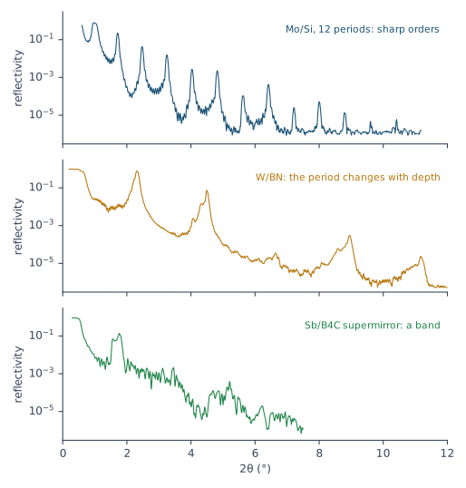
A drift (Chapter 7: A stack that drifts) and a designed gradient look the same to the curve. The difference is in what you expect. For a drift, Chapter 17: Two ways to describe a stack asks whether the stack drifts at all. For a designed gradient you know it does, and you know roughly how.
Beyond the procedure
The fitting procedure of this book separates a periodic stack from one that drifts (§9). It has no rules for a stack graded on purpose. Its limits were set on periodic stacks. This chapter follows the X-Ray Calc Help, the paper on X-Ray Calc 3 and the program’s code, and fits the two examples as they come.
Three ways to describe a graded stack
X-Ray Calc offers three ways to describe a stack whose layers change with depth. They differ in the number of free parameters. Every free parameter has to be fixed by something in the curve (Chapter 13: Why check before you fit). Table 22-1 compares them.
Table 22-1: Three descriptions of a stack whose layers change with depth. The free parameters are counted for the two models of this chapter. The paper’s own example: a Mo/Si mirror of 60 periods needs 726 variables when every layer is fitted on its own, and 18 when it is periodic. The fit times are this laboratory’s, on one GPU, at a population of 5000 and 200 iterations.
| Description | Mode | Used for | Free parameters here | Fit time here |
|---|---|---|---|---|
| one period, repeated | Periodic, or Polynomial with every box ticked | periodic mirrors | W/BN: 15 | 4 to 5 s |
| a polynomial through the periods | Polynomial | a period that changes gradually | W/BN, order 2: 19 | 4 to 6 s |
| every period on its own | Irregular | supermirrors; changes of any shape | Sb/B4C: 162 | about 30 s |
In Polynomial mode a parameter follows a polynomial in the period number, counted from the surface (Chapter 17: Two ways to describe a stack). An order-2 polynomial for the thickness of a layer costs two parameters more than a single value. In Irregular mode, every unpaired parameter has its own value in every period. A ticked box after a field pairs that parameter: it keeps one value in all the periods. Pairing is the only way to hold the count down in Irregular mode.
A gradient in Polynomial mode
Start from what you know. If the gradient is designed, enter the design before the fit. A Function profile holds a polynomial for one parameter of one layer. The fit starts its higher orders from any enabled Function profile. It starts the value at the surface, C₀, from the layer’s field.
Set the limits for the whole profile. A coefficient has no limits of its own. The program evaluates the polynomial over all N periods and keeps the whole profile inside the parameter’s Min and Max. When a profile leaves the window, the highest coefficients are set to zero, one at a time, until it fits. So the window in the Fitting Limits dialog is the range the gradient may cover. Make it wide enough for the whole design.
Keep the order low. The Order field takes 1 to 9. A larger number is read as 9. The Help advises 5 or less. Raise the order one step at a time, as Chapter 17: Raising the order does, and stop when χ² stops falling.
The W/BN mirror
The W/BN mirror is the Help’s example of a Polynomial fit (Examples → Polynomial Fitting on Graded PMMs). It was designed as 60 periods of W and BN on a W underlayer, under a BN cap. Its gradient was not designed. The laboratory record of the deposition says: “Deposition stuck after 36 pairs. Manual BN deposition ~ 240 sec.” The model in the paper has 60 periods. So this chapter fits both counts.
The model is the one in the paper’s project: a W underlayer, the W/BN stack, a BN cap and a C layer on top. It is started from the project’s values, with the project’s limits for H and σ. The densities are limited by the book’s rule, 0.7–1.0 of the bulk value in the program’s table (Chapter 15: The density ceiling). Every model was run five times. Table 22-2 gives the results.
Table 22-2: The W/BN mirror in Polynomial mode: the lowest χ² of five runs, and the period at the surface and next to the underlayer, averaged over the runs that didn’t get lost (± their standard deviation). A lost run ended above twice the best χ². σ and ρ are paired, except in the last row, where σ also follows the polynomial. Fitted by X-Ray Calc 3.9.4.1110.
| Model | N = 36: χ² | N = 36: period (Å), surface → bottom | N = 60: χ² | N = 60: period (Å), surface → bottom |
|---|---|---|---|---|
| one period | 9.16 | 39.68 | 12.54 | 39.70 |
| order 1 | 5.52 (2 runs lost) | 40.35 → 38.89 | 5.66 | 38.91 → 41.91 |
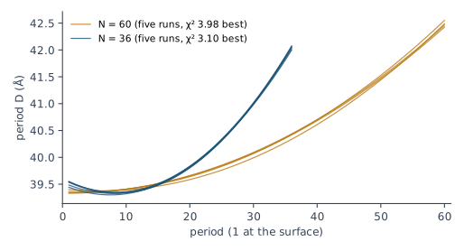
| order 2 | 3.10 | 39.51 ± 0.05 → 42.04 ± 0.03 | 3.98 (1 run lost) | 39.36 ± 0.03 → 42.48 ± 0.05 |
| order 3 | 2.87 | 39.47 ± 0.08 → 42.08 ± 0.06 | 3.95 | 39.34 ± 0.03 → 42.43 ± 0.02 |
| order 3, σ too | 3.09 | 39.88 ± 0.55 → 41.57 ± 1.23 | 3.84 (1 run lost) | 39.33 ± 0.06 → 42.60 ± 0.06 |
The period grows toward the substrate. From order 2 on, every model agrees: about 39.5 Å at the surface and 42.0 Å next to the underlayer. The runs agree to 0.1 Å or better. Order 3 lowers χ² a little further. Orders 4 and 5, in trial runs, did no better than order 3. None of them moves the profile, so order 2 is enough. The straight line of order 1 is not. With 36 periods it even gets the direction wrong.
The curve prefers 36 periods. Every model fits better with 36 periods than with 60: χ² 3.10 against 3.98 at order 2. That agrees with the deposition record. The model in the paper has 60.
Profiling σ adds nothing here. With σ on a polynomial as well, χ² stays where it was. With 36 periods the period at each end then spreads by 0.5 to 1.2 Å over the runs. The curve can’t hold both profiles, so σ stays paired.
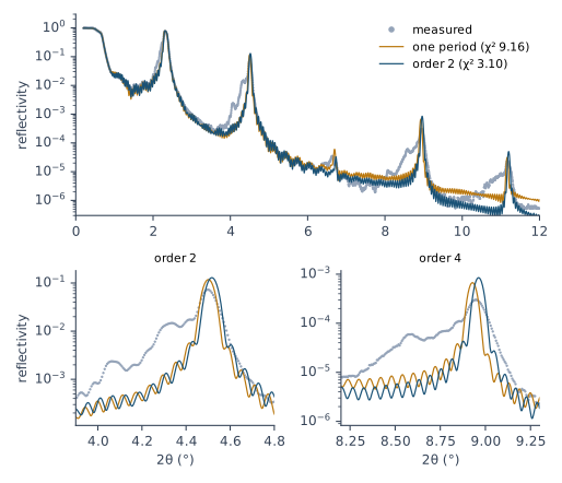
The shoulder stays. Figure 22-2 shows what the best model misses. Each order has a shoulder that reaches about 10 % lower in angle than its peak. By the Bragg law, that takes periods up to about 10 % longer than the period at the surface. The fitted profile grows by 6 %. None of the models found them. Two stacks, each with its own period, did worse (χ² 5.7 to 7.8). Orders 4 and 5 did no better than order 2. The model is too simple for this part of the curve (Chapter 19: The model is too simple). Report the period profile. Say that the shoulder is not reproduced.
Some runs get lost. Four of the 50 runs ended at more than twice the best χ², one of them at 227.6. Polynomial mode can send a run off in the wrong direction. Run every fit five times and set the lost ones aside (Chapter 16: Several runs, and their spread).
Two limits hold. In every run the BN density ended at 2.10 g/cm³, the bulk density in the program’s table. Treat it as a density on its ceiling (Chapter 20: A density on its ceiling). The top layers also end near their limits. The near-bound rule (Chapter 15: The near-bound rule) was tried: after four rounds of widening, the underlayer and the top layers still ended on their new limits. So the limits of the project were kept, and the layers above and below the stack are reported as undetermined.
A supermirror in Irregular mode
The Sb/B4C supermirror is the Help’s example of an Irregular fit (Examples → Supermirror). It has 50 periods of a mixed Sb2B4C layer, Sb and B4C, on glass, under a B4C layer and a C layer. The author’s project pairs the whole mixed layer, the densities of Sb and B4C and the σ of B4C. The thicknesses of Sb and B4C are free in every period. So is the σ of Sb. That makes 162 free parameters.
A start value on a limit. The project’s stack values sit on their lower limits, the Sb and B4C thicknesses among them. Click Run in the Fitting Limits dialog. A Warning then lists each one and asks “Proceed anyway?”. With SeedR ticked, the swarm starts spread over the whole window, so the start value matters less. Answer Yes only when that is what you want.
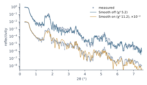
Five runs, Smooth off. The fit started from the stack’s values, with SeedR on, and took about 30 s a run. The runs ended at χ² 5.19, 5.66, 5.81, 6.52 and 7.07. The author’s fit in the paper’s project scores 7.74. Every run beat it. Each found a different minimum.
Five runs, Smooth on. They ended at χ² 11.2 to 16.7. Smooth keeps each profile smooth from period to period during the search. It pulls the periods toward each other: their standard deviation fell to 2.8–7.4 Å, against 6.8–7.9 Å with Smooth off. The band needs the spread. Figure 22-5 shows the result. With Smooth off, the fit follows the band and the structure beyond it. With Smooth on, it keeps the outline of the band and misses the structure between 2θ = 2 and 3.5°.
Where the result goes. After an Irregular fit, the structure panel shows the values of the top period. The program keeps every period in a Table item under the model, and the Thickness page draws them. From 3.9.4.1150, the GUI starts the next Irregular fit from that Table. In 3.9.4.1130 and earlier, a new Auto Fitting, or a Resume, starts every period again from the single values in the structure panel.
What the fit can tell you about each layer
The Help says of this supermirror: “The fitting revealed the designed depth-graded structure.” Five runs of the same fit don’t agree on it. Figure 22-4 plots the period of each of the 50 periods for the five runs and for the author’s fit. In depth order, the lines cross each other everywhere. Over the five runs, the thickness of a layer in a given period spreads by about 5 Å, and by never less than 1.4 Å. The layers are 10 to 30 Å thick. By the rule of Chapter 18: What the runs don’t agree on, no single layer’s thickness is a result.
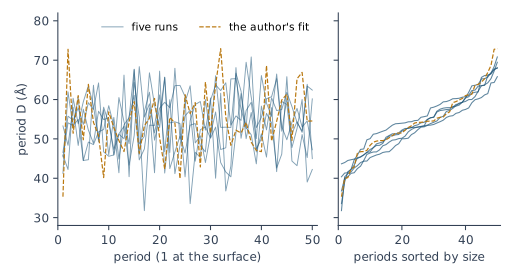
The set of periods is fixed. Sort the periods of each run by size, and the runs agree (Figure 22-4, right). In every run, and in the author’s fit, the mean period is 52 to 55 Å. The standard deviation of the periods is 6.8 to 8.0 Å. One period in ten is shorter than 42 to 46 Å. One in ten is longer than 61 to 66 Å. The total thickness of the stack agrees to about 7 %: 2586 to 2772 Å. These numbers set the band, so the curve holds them.
Runs that share a start agree with it. Five more runs started from the author’s table, period by period. They ended at χ² 6.44 to 6.86. Each period stayed near its start: the median distance from the author’s value was 0.35 Å. The runs then agree to about 1 Å in every period. That agreement comes from the start. The runs from the stack’s values reached lower χ² with other profiles.
So report what the runs agree on: the range and the mean of the periods, and the total thickness. Give the design next to them. Give a profile in depth only when runs from different starts agree on it, as they did for the W/BN mirror.
What this means when you fit
- Know what kind of stack you have. Sharp orders: periodic. Lopsided orders: a period that changes with depth. A band: a supermirror.
- Choose the description with the fewest parameters that the curve needs. One period, then a polynomial, then every period on its own (Table 22-1).
- In Polynomial mode, enter a designed gradient as a Function profile, and set Min and Max wide enough for the whole profile.
- Raise the order one step at a time, and stop when the profile stops moving.
- In Irregular mode, pair every parameter that shouldn’t change with depth. Leave Smooth off unless the design is smooth.
- Save the project after an Irregular fit. From 3.9.4.1150, the next run starts from its Table unless you choose Clear them. In 3.9.4.1130 and earlier, a new run starts from the stack’s values and ignores the Table.
- Repeat Irregular fits made with 3.9.4.1130 or earlier. They lose their pairing at the first Shake.
- Run every fit five times, from different starts. Report what the runs agree on: a profile in Polynomial mode, the set of periods and the total in Irregular mode.
- Say what the model misses, such as the shoulder of the W/BN orders.
Sources
- X-Ray Calc Help, Examples → Polynomial Fitting on Graded PMMs (the W/BN mirror; peak broadening and shape as the sign of variation across the stack) and Supermirror (the Sb/B4C supermirror in Irregular mode, “paired roughness and density”, and “The fitting revealed the designed depth-graded structure.”, quoted); Fitting → Fitting Modes, Irregular Mode, Polynomial Mode, Irregular Mode Settings (the Smoothing window, −1 automatic) and Polynomial Mode Settings; Profiles → Function Profile, Table Profile.
- Penkov et al. 2024 (J. Appl. Cryst. 57, 555–566): §2.2 and Table 1, the structure representations and the variable count of a 60-period Mo/Si mirror (726 fitted one by one, 18 periodic); §5.3 and Figure 10, the W/BN mirror in polynomial mode; §5.4 and Figure 11, the Sb/B4C supermirror in the non-periodic mode with the density and roughness of similar layers linked.
- The X-Ray Calc 3 source (build 3.9.4.1110): Polynomial mode (
XRayCalc3\LFPSO\unit_LFPSO_Poly.pas): Order + 1 coefficients per unpaired parameter of a stack with N > 1; C₀ the top period; the whole profile kept inside [Min, Max] by zeroing the highest coefficients (CheckLimitsP); higher orders started from enabled Function profiles. Irregular mode (unit_LFPSO_Irregular.pas): every period expanded; a ticked box links periods 2 to N to period 1; Smooth a moving average during the search; the top period written back to the stack and every period to the Table (unit_XRCStructure.pas); a new run starts from the stack values in 3.9.4.1130 and earlier; from 3.9.4.1150, Keep them, Resume and a reopened fitted project start each period from its Table value, a value outside the limits from the limit after a prompt, and Clear them removes the Table (X-Ray Calc session report, 2026-09-25). The Profile function editor, order 1 to 9 (Editors\editor_ProfileFunction.dfm); Select type of new extension (Forms\frm_ExtensionType.pas); Project > New extension and the Add extension button (Forms\frm_Main.dfm, release 3.9.4.1250); the prompt about extensions from the previous fitting (Units\unit_StaleExtDialog.pas); the Order field kept to 1 to 9 (Views\frame_CalcSettings.pas, release 3.9.4.1250). - The author’s records (the laboratory’s electronic notebook): the W/BN deposition, designed as 60 periods of W 1.75 nm and BN 2.65 nm on 23 nm of W under 10 nm of BN, on glass; its note “Deposition stuck after 36 pairs. Manual BN deposition ~ 240 sec.”, quoted, and its key parameter Periods 36.
- The measured curves and starting models: the project files of the paper on X-Ray Calc 3 (the W/BN mirror measured on the laboratory’s diffractometer; the Sb/B4C supermirror; the Mo/Si mirror of Figure 22-1), copied to
figures-src/ch22/. λ = 1.54043 Å and Δθ = 0.015° from those projects. - Calculated for this chapter (2026-09-25) with the X-Ray Calc 3.9.4.1110 engine, and run again with the same seeds on 3.9.4.1250 (2026-09-25), which gave the same values:
scripts/figures/ch22_engine_data.pyfits the W/BN mirror with N = 36 and 60, in five modes, five runs each with fixed seeds, population 5000, 200 iterations, SeedR on, the scale solved within 0.2, R min 5 × 10⁻⁷ (the project’s), the range from θ_max to the end of the curve, the project’s H and σ limits and the densities at 0.7–1.0 of the table’s bulk (W 19.26, BN 2.10 g/cm³). The substrate is the project’s (Si, 2.2 g/cm³); glass (2.5 g/cm³, σ 3.8 Å) gives the same profile under the 290 Å W underlayer. The near-bound widening run and the trial models (two stacks; orders 4 and 5) are inwbn-widening.jsonandwbn-probes.txt. The Sb/B4C fits were run with the engine of a build between 3.9.4.1130 and 3.9.4.1150, which carries the fix of the Irregular pairing released in 3.9.4.1150 and runs Irregular mode headless: population 5000, 200 iterations, SeedR on, the author’s pairing and limits, every parameter free (162 values), λ 1.54043 Å, Δθ 0.015°, R min 5 × 10⁻⁷, the scale solved within 0.2, the whole measured range; five fixed seeds each from the stack’s values with Smooth off, with Smooth on (window automatic), and from the author’s table (ch22_engine_data.py sb-engine,sb-engine.json). The author’s fit scores 7.74 there (the GUI of 3.9.4.1110 showed 7.81). GUI runs made earlier the same day were withdrawn: they predate the fix. Per-period spreads are sample standard deviations over the five runs.scripts/figures/fig_22_figures.pydraws Figures 22-1 to 22-5.
Cross-references: Chapter 6: The Bragg law with refraction; Chapter 7: A stack that drifts; Chapter 13: Why check before you fit; Chapter 15: The density ceiling; Chapter 16: Several runs, and their spread; Chapter 17: Two ways to describe a stack; Chapter 18: What the runs don’t agree on; Chapter 19: The model is too simple; Chapter 20: A density on its ceiling; Chapter 24: A value decided by its limit; Chapter 24: One run; Chapter 25: Does the curve fix this number, or only a sum?; Chapter 26: The number of periods; Appendix B: Menus, Buttons and Keys; Appendix D: Glossary.