Chapter 1: The four features of a curve named the plateau and the critical edge. Both come from one fact: for X-rays, the refractive index of every material is slightly less than 1. This chapter explains that fact, and where X-Ray Calc gets the numbers behind it. The formulas use θ, the grazing angle. The X-Ray Calc chart shows 2θ, so every angle you would read off the chart is also given as 2θ.
A refractive index just below 1
The refractive index n describes how a material bends a wave and how it weakens it. For X-rays it is a complex number:
δ is the refractive decrement. It sets how much the beam bends at the surface. β is the absorption index. It sets how fast the beam weakens inside the material. Both are small numbers with no unit. For silicon at the Cu Kα wavelength, λ = 1.5406 Å, δ is 7.61 × 10⁻⁶ and β is 1.73 × 10⁻⁷ (Table 4-1). So n differs from 1 only in the sixth decimal place. This book gives every length in ångströms, and 10 Å = 1 nm. So the wavelength is 0.15406 nm.
The index is below 1 because the electrons of the atoms respond to X-rays as if they were free. The photon energy is far above the binding energy of most electrons in the atom. Spiller adds the wave scattered by a thin sheet of free electrons to the incident wave. The sum looks like a wave that has passed through a slab with an index slightly below 1. The free-electron model of a metal gives the same result.
An index below 1 has a visible consequence. A beam that enters the material bends toward the surface, so its angle to the surface is smaller inside than outside (Figure 4-1, panel A). If θ is small enough, no angle inside is possible at all. The whole beam is then reflected (panel B). The section The critical angle and the plateau finds that angle.
Where δ and β come from
δ and β depend on two things: which atoms the material holds, and how many of them fill each unit of volume:
- is the classical electron radius, 2.82 × 10⁻⁵ Å.
- ρ is the density in g/cm³, A is the molar mass in g/mol, and is the Avogadro constant, 6.02 × 10²³ mol⁻¹. So is the number of atoms in each cubic centimeter.
- and are the atomic scattering factors. describes how strongly the electrons of one atom scatter. describes how strongly the atom absorbs. At photon energies well above the binding energies of the electrons, comes close to the number of electrons in the atom. Silicon has 14 electrons, and its at the Cu Kα energy is 14.30.
Three rules follow from these formulas. Each of them returns when you fit:
- δ grows in proportion to the density. A layer 10 % less dense has a δ 10 % smaller. Heavy elements have more electrons per atom and are usually denser too. So δ of W is six times δ of Si (Table 4-1).
- δ grows with λ². Away from absorption edges, changes little with the photon energy. So δ follows λ². A wrong wavelength gives a wrong δ.
- The ratio δ/β is . It does not depend on the density. Light materials absorb little: δ is 627 times β for carbon and 44 times β for silicon. For tungsten δ is only 12 times β.
The Henke tables. The values of and for 92 elements, from 50 to 30,000 eV, were tabulated by Henke, Gullikson and Davis (1993). The tables combine measured absorption data with theory, and is calculated from . They smooth over the fine structure close to an absorption edge, so a value near an edge can be wrong. Cobalt at the Cu Kα energy is such a case. The Co K edge is at 7708.8 eV, 339 eV below the Cu Kα energy.
X-Ray Calc stores one Henke table for each material. The table holds and against the photon energy E, the molar mass, and the bulk density. For the calculation, the program converts λ to the energy, E = 12398.6/λ eV with λ in Å. Then it reads and by linear interpolation between the two nearest rows of the table. A layer with ρ = 0 is calculated with the bulk density from its table. A compound is a table of its own, such as SiO2 or B4C. Tools > Create new material … makes a new one from elements or existing materials.
Here is δ of silicon at λ = 1.5406 Å, from the X-Ray Calc table Si. The table gives ρ = 2.332 g/cm³ and A = 28.086 g/mol. Its row at 8048.79 eV gives = 14.297 and = 0.32485.
- The number of atoms: = 2.332 × 6.02 × 10²³ / 28.086 = 5.00 × 10²² atoms per cm³. One cm³ holds 10²⁴ ų, so this is 0.0500 atoms per ų.
- The prefactor: λ²/2π = 2.82 × 10⁻⁵ × 1.5406² / 2π = 1.065 × 10⁻⁵ ų.
- δ = 1.065 × 10⁻⁵ × 0.0500 × 14.30 = 7.61 × 10⁻⁶.
- β = 1.065 × 10⁻⁵ × 0.0500 × 0.325 = 1.73 × 10⁻⁷.
X-Ray Calc gives δ = 7.609 × 10⁻⁶ and β = 1.729 × 10⁻⁷. Table 4-1 lists the same numbers for eight materials that often appear in multilayers and substrates.
Table 4-1: Optical constants and critical angles at λ = 1.5406 Å, calculated by X-Ray Calc from its own Henke tables at the bulk density of each table (ρ = 0 in a layer). 10⁶ δ = 7.61 means δ = 7.61 × 10⁻⁶. θc = √(2δ), converted to degrees; 2θc is where the edge appears on the X-Ray Calc chart.
| Material | Bulk ρ (g/cm³) | 10⁶ δ | 10⁶ β | δ/β | θc (°) | 2θc (°) |
|---|---|---|---|---|---|---|
| C | 2.266 | 7.28 | 0.0116 | 627 | 0.219 | 0.437 |
| B4C | 2.52 | 7.53 | 0.00653 | 1150 | 0.222 | 0.445 |
| Si | 2.332 | 7.61 | 0.173 | 44.0 | 0.224 | 0.447 |
| SiO2 | 2.65 | 8.60 | 0.111 | 77.5 | 0.238 | 0.475 |
| Co | 8.79 | 23.54 | 3.41 | 6.91 | 0.393 | 0.786 |
| Mo | 10.22 | 28.66 | 1.88 | 15.3 | 0.434 | 0.868 |
| Ru | 12.437 | 34.76 | 2.57 | 13.5 | 0.478 | 0.956 |
| W | 19.263 | 46.33 | 3.87 | 12.0 | 0.552 | 1.103 |
Going Deeper: the formula inside X-Ray Calc
X-Ray Calc works with the dielectric constant ε = n², which for small δ and β is
For each layer the program computes and , with ρ in g/cm³, λ in Å and = 0.54014 × 10⁻⁵. This constant is , converted to these units. So the program’s formula is the formula of this section, multiplied by 2.
The critical angle and the plateau
Snell’s law links the angle of the beam inside the material, , to the angle outside, θ. At grazing angles, with the absorption left out, it becomes
with both angles in radians. Above a certain angle, is real, and part of the beam enters the material. Below it, would be negative, so no beam can enter. That angle is the critical angle:
For silicon, = 0.00390 rad = 0.224°. On the X-Ray Calc chart the edge of a bare silicon surface is at 2θ = 0.447°. δ grows with ρλ², so grows with λ√ρ. A layer 20 % less dense has a critical angle about 10 % smaller. Table 4-1 gives for all eight materials. Spiller lists 0.223° for Si, 0.435° for Mo and 0.555° for W at 1.54 Å. The values agree closely.
Below nearly the whole beam is reflected, and the curve forms the plateau (Figure 4-2). The plateau is never quite at 1. Absorption takes a small part of the beam. The part grows as the angle comes close to . Absorption also rounds the edge. A material with a large δ/β has a sharp edge. At 0.9 a bare silicon surface still reflects 91 % of the beam, and tungsten reflects 72 %. At itself the values are 65 % and 45 %.
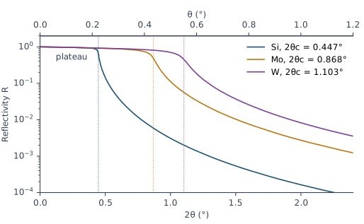
Which δ sets the edge of a coated sample? A real sample is rarely one material. The edge then belongs to the top part of the sample as a whole. The demo multilayer of Chapter 3: The example shows this. Take its layers without the thickness gradient: a 50 Å Si cap on 30 periods of 25 Å Si and 15 Å Mo, all smooth. The average δ of one period, δ̄, is 1.55 × 10⁻⁵, and = 0.319°. X-Ray Calc puts the edge of this stack between θ = 0.30° and 0.33° (2θ = 0.60–0.66°). There its reflectivity falls from 0.72 to 0.19. The Si cap alone would put the edge at θ = 0.224°. The edge of the whole sample follows the average δ of the stack under the cap. Chapter 6: The Bragg law with refraction uses the same average in the Bragg law.
On a measured curve the plateau also falls at the smallest angles. There part of the beam misses the sample, as Chapter 1: The four features of a curve explains. Chapter 10: Is This Curve Worth Fitting? checks for it.
Why the curve falls so steeply above the critical angle
Above the beam enters the material. Only a small part of it is reflected. Well above the reflectivity of a smooth surface is
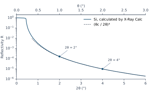
Here 2θ is twice the grazing angle, the number on the X-Ray Calc chart. So each doubling of the angle divides R by 2⁴ = 16. For bare silicon the formula gives 1.56 × 10⁻⁴ at 2θ = 2° and 9.75 × 10⁻⁶ at 2θ = 4°. X-Ray Calc calculates 1.64 × 10⁻⁴ and 9.86 × 10⁻⁶ (Figure 4-3). Close to the formula is too low, and there you need the full calculation.
This fast fall is the reason an XRR curve is always plotted on a logarithmic axis. Between 2θ = 1° and 6°, the reflectivity of bare silicon falls by more than three orders of magnitude. A multilayer adds its Bragg orders on top of this fall. The fall itself remains. The measured curve in Chapter 1: Figure 1-2 spans more than five orders of magnitude.
A rough surface makes the curve fall faster than . That extra fall is where roughness shows on a curve. Chapter 7: A boundary with a width explains it.
Going Deeper: the reflection coefficient of one surface
At grazing angles the amplitude reflection coefficient of a surface, seen from vacuum, is
with θ in radians. It is the Fresnel formula for s-polarization, written for small angles. Below the square root is nearly imaginary, so |r| is close to 1. Far above , the square root is close to θ − δ/θ, and r ≈ δ/(2θ²) = . Squaring gives . For p-polarization the formula differs, but below θ ≈ 3° the result differs by less than 0.5 % (X-Ray Calc Help, Calculation → Polarization). X-Ray Calc does not use this approximation. It calculates the exact reflection of the whole structure. Chapter 8: From the substrate up: the recursion explains how.
What this means when you fit
The critical edge carries δ of the top part of your sample. δ carries its density. The edge also sits next to the plateau, the region where the measured curve is put on the reflectivity scale. So the edge must be inside the fitting range. Start the fitting range at , the measured maximum just below the edge. Chapter 14: Where the fitting range starts and ends sets it. After the fit, Chapter 18: The edge compares the calculated edge with the measured one.
Two more points follow from this chapter:
- The material is never fitted. X-Ray Calc takes and from the Henke table of each material. A fit can change δ and β of a layer only through its density.
- The wavelength sets δ. δ grows with λ², so grows with λ. Take the wavelength from your measurement file, as Chapter 10: The wavelength comes from the file shows.
Sources
- Spiller, E. (1994). Soft X-ray Optics. SPIE. The index n = 1 − δ + iβ and its sign convention (p. 6, Table 2.1); the index below 1 from the wave scattered by free electrons, and the same result from the free-electron model (pp. 7–10, Eqs. 2.4–2.16); δ and β in terms of , , the density and the atomic weight (p. 13, Eqs. 2.17–2.18), with r₀ = 2.82 × 10⁻¹³ cm (p. 8) and 6.02 × 10²³ atoms per mole (p. 13); approaching the number of electrons per atom (pp. 7, 9) and δ ∝ λ² at high energy (p. 16); the Henke tables and their errors near absorption edges (pp. 11–16); Snell’s law and the angle inside a material (pp. 23–24, Eqs. 3.2 and 3.5); the critical angle, sin θc ≈ √(2δ) (p. 25, Eqs. 3.7–3.8); the reflectivity well above the critical angle, R = q_c⁴/16q⁴ (p. 26, Eq. 3.11), which the chapter writes as (θc/2θ)⁴; a sharp edge only for small β/δ, and a fall faster than q⁻⁴ for a rough surface (pp. 29–30); the plateau below 100 % because of absorption (p. 32); θc at 1.54 Å for Si, Mo and W (p. 34, Table 3.1). Spiller measures angles from the surface normal and writes r₀ for the electron radius; the chapter uses the grazing angle θ and writes . The condition printed with Eq. 3.12, “θ₀ ≪ θcr”, reads ≫ in the derivation on the same page; the chapter does not use Eq. 3.12.
- Henke, B. L., Gullikson, E. M. & Davis, J. C. (1993). X-ray interactions: photoabsorption, scattering, transmission, and reflection at E = 50–30,000 eV, Z = 1–92. Atomic Data and Nuclear Data Tables 54, 181–342. The tabulated and , their range, and determined from the absorption data (abstract).
- X-Ray Calc Help: Calculation → Algorithm (ε = 1 − 2δ + 2iβ; δ and β proportional to ρλ²f₁/A and ρλ²f₂/A; the Henke tables interpolated linearly in E = 12398.6/λ eV) and Polarization (s and p within 0.5 % below θ ≈ 3°); Models → Density 0 and the substrate density (ρ = 0 means the bulk density; the
SiO2table holds crystalline quartz, 2.65 g/cm³; enter 2.2 g/cm³ for fused silica); Tools → Create New Material, Edit Henke Table. - The X-Ray Calc 3 source: the dielectric constant of each layer, with the constant 0.54014 × 10⁻⁵ (
Shared\Math\unit_materials.pas:90, 249–251); the Henke table read and interpolated at E = H/λ, with H = 12398.6 eV·Å (Shared\Math\math_globals.pas,ReadHenke); the Henke table editor and its labels, with the molar mass labeled A (g/mol) from 3.9.4 build 1030 and N (a.u.) before (XRayCalc3\Editors\editor_HenkeTable.dfm,.pas); the menu command Edit Henke table… (XRayCalc3\Forms\frm_Main.dfm); s-polarization as the default (frame_CalcSettings.dfm). - Calculated for this chapter (2026-09-24, rerun 2026-09-25) with the X-Ray Calc 3.9.4.1250 engine, at λ = 1.5406 Å: δ, β and the Co K edge for Table 4-1; the curves of Figures 4-2 and 4-3 and the demo-layer stack, with σ = 0, no resolution blur and s-polarization.
scripts/figures/ch4_engine_data.pyruns the calculations and keeps the results infigures-src/ch4/.scripts/figures/fig_4_curves.pydraws the figures and computes θc = √(2δ) and every reflectivity value quoted in the text. The Si example and the fused-silica values in the Warning are computed on the page from the Henke table values.
Cross-references: Chapter 1: The four features of a curve; Chapter 3: The example; Chapter 5: What density does to the fringes; Chapter 6: The Bragg law with refraction; Chapter 7: A boundary with a width; Chapter 8; Chapter 10; Chapter 12; Chapter 14: Where the fitting range starts and ends; Chapter 15: The density ceiling; Chapter 18: The edge; Appendix A: Notation and Units; Appendix C: Where Optical Constants Come From; Appendix D: Glossary.