A single film on a substrate is the usual way to calibrate a deposition rate. Deposit one material for a known time, measure the film, and divide. This chapter fits two such films by the rules of the fitting procedure: a carbon film on glass and a cobalt film on glass. Both were deposited in the same laboratory as the Co/C multilayers of the earlier chapters. Chapter 5: Reading a thickness from the fringes read the thickness of the carbon film from its fringes. This chapter fits it.
What one film tells you
The fitting procedure is strict about a film of the light material: “A single film of the light material of the design, on the substrate, gives its thickness, and from it the deposition rate, and nothing else: report its sigma and density as undetermined.” (§12.1)
The reason is in the fringes. Their positions fix the thickness. Their depth depends on the density of the film and on the roughness of both of its boundaries at once (Chapter 5: What this means when you fit). A carbon film on glass is a weak pair. The two have similar δ, so the fringes are shallow and the three effects can’t be told apart.
The single-film exceptions
A film is fitted with a few settings of its own. Table 21-1 sets them beside the settings of a multilayer.
Table 21-1: The settings that differ for a single film, from the fitting procedure and one laboratory’s preset. The reasons are the procedure’s.
| Setting | Multilayer | Single film | Why |
|---|---|---|---|
| Start of the range | θmax, the edge included | θ = 0.3° (2θ = 0.6°), for a film of the light material | the model shows a feature at the edge that the data don't have (§6.3) |
| End of the range | at least the first seven predicted orders | past the last fringe that stands 3 times above the background | a film has no orders (§6.4) |
| σ limits | 1–8 Å | 1–10 Å | the preset's value for a film |
| Population | 5000 | 2000 | the preset's value for a film |
| Weighting | θ weight off, peak weight on | the same | the preset |
| Polynomial fit | always, after the fit with one period | none | a film has no periods (§9.2) |
| Report | H, σ and ρ, with their spreads | H only; σ and ρ undetermined, for a film of the light material | §12.1 |
Everything else stays as for a multilayer: the solved scale, R min at one count, smoothing off, the Δθ scan, five runs and the near-bound rule (Chapter 14 to Chapter 16).
The edge of a carbon film
The first exception comes from the author’s own fits. In the author’s words: “The problem of single layer carbon and X-Ray Calc: we often have this artifact. So I trimmed to 0.6. But only for single carbon; in other cases it works fine.”
Figure 21-1 shows it on the carbon film. A one-layer model was fitted twice: once with the range from θ_max, and once from θ = 0.3°. On the lower part of the edge, over 2θ = 0.44–0.52°, both calculated curves stay above the data. With the edge in the range, the edge check of Chapter 18: The edge reads 0.95, 1.38 and 0.86, so the middle point misses by 38 %. The paper on the procedure records the same miss in an earlier fit: 0.127 calculated against 0.073 measured, at θ = 0.26°.
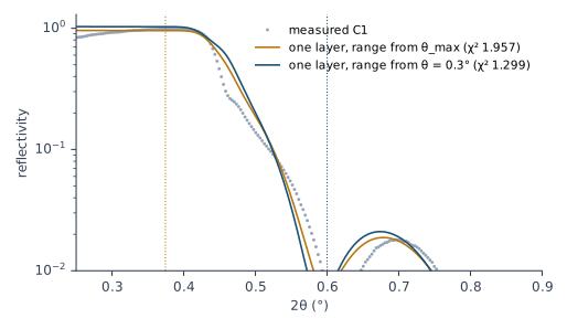
Neither fit can match the edge, and the rest of the curve pays for trying. So the procedure moves the start past the edge for a film of the light material. The thickness hardly notices: 307.1 Å with the edge in the range, 307.3 Å without it.
Fitting the carbon film
The procedure’s model for the carbon film is one C layer with the contamination layer above it (Chapter 7: The dirty surface). The author’s comment on a one-layer fit of this film was: “Is bad, because it’s not possible to fit a single-layer carbon with a single-layer model. For metals it works nice, but not for carbon. It needs something lighter on top.” Table 21-2 gives the fits with and without the contamination layer.
Table 21-2: The carbon film C1 (deposited for 1000 s), fitted by the single-film rules: the run with the lowest χ², with the spread over five runs where it is larger than the last digit. Δθ = 0.015° by the scan. Fitted by X-Ray Calc 3.9.4.1270.
| Model | Range from | χ² | Film: H (Å), σ (Å), ρ (g/cm³) | Contamination layer: H (Å), ρ | Total H (Å) |
|---|---|---|---|---|---|
| one C layer | θmax | 1.957 | 307.1, 7.41, 1.94 | none | 307.1 |
| one C layer | θ = 0.3° | 1.299 | 307.3, 7.41, 1.86 | none | 307.3 |
| C layer + contamination layer | θ = 0.3° | 1.170 | 299.8 ± 0.1, 0.10, 1.83 | 13.0, 1.00 | 312.7 ± 0.1 |
The contamination layer lowers χ² from 1.30 to 1.17. The film comes out at 299.8 Å under 13.0 Å of contamination. That agrees with the laboratory’s own refit of the same curve, 300.5 Å under 13 Å. The five runs agree on the thicknesses to 0.1 Å and on the densities to 0.01 g/cm³.
The two models don’t agree. The σ of the film goes from 7.41 Å to 0.10 Å, and the film thickness from 307.3 to 299.8 Å. The runs agree with each other, so the spread is small. The model sets the value. This is the lesson of Chapter 20: The runs agree, the models don’t, now for σ. Report σ and ρ as undetermined, as §12.1 says. The film’s σ of 0.10 Å also sits on its lower limit of 0, after the near-bound rule moved that limit down from 1 Å.
The thickness and the rate. The film was deposited for 1000 s. So its rate is 299.8 / 1000 = 0.300 Å/s. The one-layer model would give 0.307 Å/s. The 2 % comes from the choice of model. The contamination layer belongs in the model you report.
What the fit can’t match
No model of this film matched both its edge and its fringe contrast. The paper on the procedure says so for every attempt, by the author and by the test sessions: “No model of the single carbon film C1, by the expert or by any session, reproduced both its critical edge and its fringe contrast. The film yields its thickness, and nothing further.” After nine failed attempts the author’s words were: “I don’t found good model for carbon.”
The procedure warns against two repairs: “Do not try to repair that with the resolution (section 8) or the substrate roughness (section 2); neither is the cause.” (§12.2) Both move the fringe depth, so a fit can use them to hide the miss. Keep Δθ from the scan and the substrate as Chapter 12 sets it. Report the thickness, and say that the edge and the fringe contrast are not reproduced.
A metal film and the layers on top
The procedure says that “The metal films fit with a one-layer model.” (§12.2) The cobalt film of this chapter doesn’t. It was deposited on glass for 800 s, measured in the same way, and fitted by the same rules. The range starts at θ_max. Table 21-3 gives three models.
Table 21-3: The cobalt film P2-08 (deposited for 800 s): the run with the lowest χ², with the spread over five runs where it matters. Δθ by the scan: 0.015° for the first two models, 0.013° for the third. At 0.015° the first run of the third model gave χ² = 2.488. Fitted by X-Ray Calc 3.9.4.1270.
| Model | χ² | Co: H (Å), σ (Å), ρ (g/cm³) | Layers on top: H (Å), ρ (g/cm³) | Sum on top (Å) |
|---|---|---|---|---|
| one Co layer | 6.331 | 296.9, 13.79, 8.35 | none | none |
| Co + contamination layer | 2.389 | 291.0, 8.45, 8.42 | C 22.2, 2.40 (on its limit) | 22.2 |
| Co + CoO + contamination layer | 2.463 (runs to 2.527) | 289.5 ± 0.6, 6.5 ± 0.3, 8.52 | CoO 15.8 ± 1.3, 4.46; C 9.8 ± 1.1, 1.69 | 25.6 ± 0.6 |
Figure 21-2 shows the measured curve with the three fits. Above 2θ = 2.5° the one-layer curve has almost no fringes left, while the measured fringes run on to the end of the range. The two models with layers on top follow them, and on this scale they can’t be told apart.
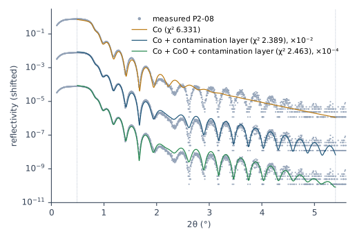
One Co layer misses by far: χ² = 6.33. Its σ went past the film limit of 10 Å to 13.8 Å, after the near-bound rule widened it. A roughness that large stands in for something the model lacks (Chapter 19: The model is too simple).
A contamination layer on top brings χ² to 2.39. But its density climbed through each widened limit and ended at 2.40 g/cm³, at 22 Å. That is the laboratory’s ceiling for sputtered carbon (Chapter 15: The density ceiling). Carbon contamination from the air is light. A layer of 22 Å at the density of sputtered carbon is not contamination. It stands in for a denser layer.
Cobalt oxide under the contamination layer is the model of the laboratory’s fit of record for this film. It gives χ² = 2.46, about the same as the dense carbon layer. The curve doesn’t choose between them. What it does fix is the sum of the layers above the metal: 25.6 ± 0.6 Å, while the oxide and the contamination layer spread by 1.3 and 1.1 Å on their own. Report the sum, with the split undetermined (Chapter 18: Two layers as a sum). The X-Ray Calc Help shows the same kind of case: a TiZrNi coating fitted first with a TiO2 layer on top, then with further surface layers, which lowered its cost function from about 0.48 to 0.14 (Examples → Single-Layer Coating).
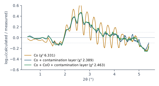
Figure 21-3 shows the same through the residual. The one-layer residual swings through every fringe, because its total thickness is wrong. The other two lie on top of each other. All three share a stretch from 2θ = 2.0 to 3.3° where the model runs about +0.3 above the data. No model here removes it. X-Ray Calc draws this residual too, point by point, in the strip under the chart (Result > Residual strip; Chapter 18: The residual by band). The figure averages it over 61 points, so that the level of each stretch shows.
The thickness and the rate. The Co layer comes out at 289.5 Å with the oxide and 291.0 Å with the dense carbon layer. The one-layer model gives 296.9 Å. Divided by 800 s, the two models with a top layer give 0.362 and 0.364 Å/s. The laboratory’s fit of record gave 288.65 ± 1.62 Å for the metal, 0.361 Å/s. So the rate is fixed to about 1 %, whatever sits on top, once something does.
Reporting a film
A film’s report is short:
- the thickness of the film, with its spread over the runs, and the model it was fitted with;
- the total of the layers on the substrate, and the sum of the layers on top when their split is undetermined;
- the deposition rate: the thickness divided by the deposition time from the deposition record;
- σ and ρ of a film of the light material, reported as undetermined;
- the range start and why, and any part of the curve the model doesn’t reproduce, such as the edge or the fringe contrast of a carbon film.
Chapter 23: Writing the numbers puts these items into the report.
What this means when you fit
Report a single film as a thickness and a rate. σ and ρ of a light film are undetermined.
Start the range at θ = 0.3° for a light film, past the edge its model can’t match. Keep θ_max for a metal film.
Put the contamination layer on every film, and a layer that can grow on a metal, such as its oxide. Report what the curve fixes: the metal, and the sum on top.
Don’t repair a misfit with the resolution or the substrate σ. Say which part of the curve the model misses.
Sources
- Fitting procedure (Penkov, Peng & Fu 2026): §12.1, a single film of the light material gives its thickness and nothing else, quoted; §12.2, a one-layer model misses the edge and the fringe contrast, the two repairs not to try, quoted, and “The metal films fit with a one-layer model.”, quoted; §12.3, the exceptions in the preset; §6.3, the range start for a single film of the light material and its reason; §6.4, the range end for a film; §7.2, the σ limits for a single film; §8.5–8.6, the weighting and the population for a single film; §9.2, no profile fit for a single film; §10.8, a sum reported when the split is undetermined.
- The procedure’s preset (
skill-v5\presets\csmic-empyrean.json), one laboratory’s values:single_film.theta_min_deg0.3,single_film.sigma_bounds_A1–10;chi2.single_film(θ weight 0, point weight on);optimizer.population.single_film2000; the contamination layer (C, 15 Å, σ 3 Å, 0.9 g/cm³; 5–40 Å, 1–10 Å, 0.6–1.4 g/cm³);materials.named(C 1.5–2.4, Co 6.0–8.79);materials.default_rule(CoO at 0.7–1.0 of its table’s 6.2 g/cm³). - The expert’s rulings (Supplementary S3): ruling 34 and 35, the artifact at the edge of a single carbon film and the start moved to 2θ = 0.6°, quoted; ruling 36, a single carbon film needs something lighter on top, quoted; ruling 54, no good model for carbon, quoted.
- The methods paper on the procedure (Penkov, Peng & Fu 2026, arXiv:2609.28926): §3–4, the procedure written down while the author fitted the carbon film in the program; §6, the baseline miss at the edge of that film (0.127 calculated, 0.073 measured, θ = 0.26°); Supplementary S4.6, the refit at 300.5 Å under 13 Å of contamination; S4.7, no model reproduced both the edge and the fringe contrast, quoted.
- The author’s records (the laboratory’s electronic notebook): the carbon film P2-06, C(260917B), deposited for 1000 s; the cobalt film P2-08, Co(260921A), deposited for 800 s, measured on 2026-09-22; the fit of record of the cobalt film under procedure v5 (engine 3.9.2.970): Co 288.65 ± 1.62 Å, CoO 15.0 ± 3.8 Å, C 11.6 ± 4.4 Å, their sum 26.65 ± 0.80 Å, Co rate 0.361 Å/s for the metal alone. The first fit of that film found the contamination layer’s density on its limit and a residual of +0.305 in one band without the oxide.
- X-Ray Calc Help, Charts → Residual Strip (the residual drawn under the chart, point by point); Examples → Single-Layer Coating (a TiZrNi coating with a TiO2 layer, then surface layers, cost about 0.48 then 0.14; from Penkov et al. 2024, Figure 5).
- Calculated for this chapter (2026-09-25) with the X-Ray Calc 3.9.4.1030 engine, and run again with the same seeds on 3.9.4.1270 (2026-09-25), which gave the same values:
scripts/figures/ch21_engine_data.pyfits the two films by the rules of Table 21-1, five runs each with the preset’s seeds, 200 iterations, λ = 1.541874 Å, the scale solved within 0.2, R min at one count, the range ends of the laboratory’s v5 refits (θ = 1.6775° for the carbon film, 2.7° for the cobalt film), Δθ from a one-run scan over 0.012–0.015°, and two rounds of the near-bound rule; the substrate is SiO2 at 2.50 g/cm³, σ 3.8 Å (Chapter 12). The results and the figures’ curves are infigures-src/ch21/(fits.json,curves.json,numbers.txt);scripts/figures/fig_21_figures.pydraws Figures 21-1 to 21-3. The rates are computed on the page from the fitted thicknesses and the deposition times. - The measured curves: the carbon film C1 from the fitting procedure’s data deposit (CC BY 4.0); the cobalt film P2-08 from the author’s measurement.
Cross-references: Chapter 5: Reading a thickness from the fringes; Chapter 7: The dirty surface; Chapter 12: The top of the stack; Chapter 14: Trimming the data to the range; Chapter 16: Several runs, and their spread; Chapter 18: Two layers as a sum; Chapter 18: The residual by band; Chapter 19: The model is too simple; Chapter 20: The runs agree, the models don’t; Chapter 23: Writing the numbers; Chapter 24: A layer that stands in for a missing one; Chapter 25: Does the curve fix this number, or only a sum?; Chapter 26: The layers in the model.