A multilayer repeats the same layers many times. Its curve has tall peaks, the Bragg orders, on top of the fall described in Chapter 4: Why the curve falls so steeply above the critical angle. Their positions give the period. Their heights depend on how the period is shared between the layers, on the roughness, and on how regular the stack is. This chapter builds on the single film of Chapter 5: Two reflections, one film. The worked example is the measured Co/C multilayer of Chapter 1: Figure 1-2.
A stack that repeats
A periodic multilayer mirror (PMM) is a stack of N identical periods. Each period holds the same layers, for example 31 Å of C over 19 Å of Co. The period D is the sum of the layer thicknesses H of one period. In X-Ray Calc such a stack is one block of the structure panel, and the number at the right of its title is N.
Every period reflects a small part of the beam. The wave reflected one period deeper travels an extra distance of 2D sin θ (Figure 6-1). When this extra distance is a whole number m of wavelengths, the waves from all N periods add. This gives the Bragg order m:
This is the plain Bragg law. For a period of 50 Å at λ = 1.5406 Å, the first order is near θ = λ/2D = 0.0154 rad = 0.88°, so near 2θ = 1.76° on the chart.
The top and the bottom of the whole stack still give Kiessig fringes, as a single film does. Their thickness is the total N·D. So the fringes between two orders are N times closer than the orders. For a smooth Co/C stack of 50 Å periods, X-Ray Calc puts 18 fringe maxima between the first and second orders when N = 20, and 8 when N = 10. That is N − 2 in both cases. The measured curve of Chapter 1: Figure 1-2, panel B, shows these fringes.
The Bragg law with refraction
The plain law ignores refraction. Inside the stack the beam travels at a smaller angle than outside (Chapter 4: A refractive index just below 1). The extra distance follows the angle inside. With this correction the order positions are
Here δ̄ is the δ of the period averaged over its layers, each weighted by its thickness. It is the same average that sets the critical edge of the stack (Chapter 4: The critical angle and the plateau). The term 2δ̄ is a fixed amount added to sin²θ. It moves the first order most. At high orders it hardly matters.
Table 6-1 lists the four orders of the measured Co/C curve. The third column gives the period that the plain law returns from each order on its own. The values grow from 48.29 Å to 50.22 Å. They approach the true period as m grows, the way the film thickness did in Chapter 5: Table 5-1.
Table 6-1: The Bragg orders of the Co/C multilayer of Chapter 1: Figure 1-2. Each position is the highest measured point of the order. D from the plain law is mλ/(2 sin θm), with λ = 1.541874 Å, the wavelength the measurement file gives. The last two columns predict each order from the first: evenly spaced, as m times 2θ₁, and from the Bragg law with refraction fitted to all four orders.
| Order m | 2θ measured (°) | D from the plain law (Å) | 2θ evenly spaced (°) | 2θ with refraction (°) |
|---|---|---|---|---|
| 1 | 1.8295 | 48.29 | 1.8295 | 1.847 |
| 2 | 3.5515 | 49.76 | 3.6590 | 3.558 |
| 3 | 5.3185 | 49.85 | 5.4885 | 5.298 |
| 4 | 7.0405 | 50.22 | 7.3180 | 7.048 |
A least-squares fit of the four positions for D and δ̄ gives D = 50.34 Å. The expert’s full fit of this curve has 31.21 Å of C and 18.82 Å of Co, a period of 50.03 Å. It was made at λ = 1.5406 Å, which puts the period 0.08 % lower (Chapter 10: The wavelength comes from the file). The law is an approximation. The fit calculates the whole curve. The two periods differ by 0.6 %.
Going Deeper: the period from the orders without a fit program
Write for the period that the plain law gives from order m. The law with refraction can then be written as
So the points plotted against lie on a straight line. The line meets the vertical axis at . Any spreadsheet can fit it. For the four orders of Table 6-1 the line gives D = 50.23 Å. Two orders are enough to solve for D and δ̄ directly, but more orders give a steadier result. The same method works for the fringes of a single film, as in Chapter 5: Reading a thickness from the fringes.
Why evenly spaced orders mislead you
It is tempting to place the orders at 1, 2, 3, 4 times the first one. The fourth column of Table 6-1 does this. Every higher order then lands too high, and the error grows with m. The 2nd order is predicted 0.107° too high in 2θ, and the 4th 0.277° too high. That is 16 % of the spacing between orders. The column with refraction stays within 0.021° of every measured order.
The error grows with the period, because the orders come closer together. Figure 6-2 shows a Co/C stack with D = 100 Å. Its orders are about 0.87° apart in 2θ. The evenly spaced marks drift to the right. The mark for m = 5 lands on the 6th order. From there on each evenly spaced mark sits on the next order. The Bragg law with refraction matches the calculated orders within 0.008° from the 2nd order on. It misses the first order by 0.046°. The first order is strong. There the law is least exact.
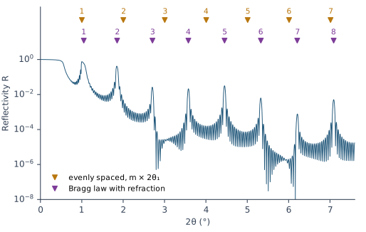
A wrongly numbered order gives a wrong period. It also gives a wrong fitting range. The fitting procedure puts it this way: “a misassigned order corrupts both the period and the fitting range”.
The layer ratio: weak and missing orders
The layer ratio Γ is the thickness of the heavy layer divided by the period. For the Co/C curve of Table 6-1, Γ = 18.82/50.03 = 0.376. Each period has two interfaces: light on heavy, and heavy on light. They reflect with opposite signs. At order m the reflections from all periods are in phase. The two interfaces within one period, though, are in phase only for some values of Γ. The strength of order m follows
When mΓ is a whole number, the two interfaces cancel, and order m nearly disappears. A ratio of 0.5 removes the even orders. A ratio of 1/3 removes the 3rd and the 6th. The factor is the same for Γ and 1 − Γ. So the orders alone can’t tell you which layer is the thicker one.
Figure 6-3 shows three smooth Co/C stacks with the same period of 50 Å:
- Γ = 0.5. The 2nd order is 60 times weaker than the 3rd, although it lies at a smaller angle.
- Γ = 1/3. The 3rd order is 150 times weaker than the 4th. The 6th almost disappears too.
- Γ = 0.376, the ratio of the measured stack. The factors for m = 1 to 4 are 0.86, 0.49, 0.15 and 1.00. So the 3rd order is weak. The 4th stands above it.
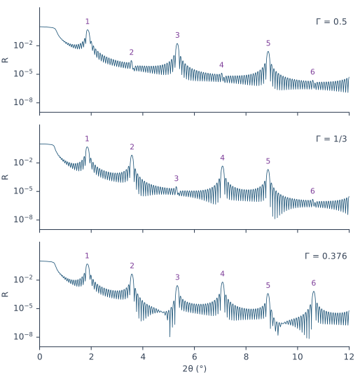
The orders don’t vanish completely. The sin² rule treats each reflection as small and ignores refraction. The full calculation leaves a trace of each missing order.
The higher orders carry the fine details
The fitting procedure states this as a rule for reading a curve: “Larger diffraction orders carry the smaller details. The first order fixes little beyond the period; the higher orders carry the layer ratio, the interface widths and any drift through the stack.” Three effects lie behind the rule:
- Roughness. Roughness weakens a reflection more at larger angles (Chapter 5: What roughness does to the fringes). So a small change of σ hardly touches the first order and strongly changes the high orders.
- The layer ratio. The factor sin²(mπΓ) changes faster with Γ when m is large.
- Drift. When the period changes through the stack, each period puts its order m at a slightly different angle. The spread in angle grows with m. So a drift widens and lowers the high orders first.
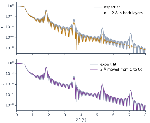
Figure 6-4 shows the first two effects on the fitted model of the measured Co/C stack. Adding 2 Å to the roughness of both layers lowers the 1st order to 0.70 of its height. It lowers the 4th order to 0.013. Moving 2 Å from C to Co changes the ratio from 0.376 to 0.416 at the same period. The 1st order rises by 3 %. The 2nd falls to 0.55 of its height. The 3rd rises to 1.8 times its height.
What this means when you fit
Take the period from the curve before the first fit. In Periodic mode X-Ray Calc keeps the period of each stack at its start value. The fit moves thickness between the layers of a period but keeps their sum. Free period ± lets the period move, but only within a window around the start. So the start period must already be close. Get it from the orders with the Bragg law with refraction. Polynomial mode lets the period change. Chapter 11: Numbering the orders reads the orders, and Chapter 12: The periodic stack uses the period. Chapter 17: Periodic or Polynomial? A Stack That Drifts compares the two modes.
Number every order, including the missing ones. A missing order keeps its number (The layer ratio: weak and missing orders). The numbered orders, seen and predicted, also set the end of the fitting range (Chapter 14: Where the fitting range starts and ends).
Judge a fit on the orders first. The fitting procedure’s first rule for reading a curve is “Peaks have priority.” Order positions test the period. Their heights, and above all the heights of the high orders, test the layer ratio and the roughness. Between the orders, the level depends on the ends of the stack: the top layer and the substrate side. Chapter 7: The dirty surface: a contamination layer covers them. Chapter 13: The variants and what they move maps each parameter to the part of the curve it moves. Chapter 18: The order table checks the orders one by one.
Sources
- Fitting procedure (Penkov, Peng & Fu 2026), §1.5: predict each order with sin²θm = (mλ/2d)² + 2δ, match the measured maxima, refine d and δ by least squares and repeat until the matching stops changing; “Spacing the orders linearly as m·θ_1 misassigns the high orders, because refraction shifts them, and a misassigned order corrupts both the period and the fitting range (section 6).” §3.3: the two rules “Peaks have priority” and “Larger diffraction orders carry the smaller details”. §9.6: the Polynomial (profile) fit lets the period float. The procedure writes d for the period; the book writes D.
- The measured curve CoC5 (record P2-05, a Co/C multilayer of 20 periods on glass) and its expert fit (
fits/CoC5-expert.xrcx: 31.2135 Å C, σ 4.3254 Å, ρ 2.0621 g/cm³; 18.8183 Å Co, σ 5.7386 Å, ρ 6.2509 g/cm³; substrate SiO2, σ 3.8 Å, ρ 2.65 g/cm³) are from the fitting procedure’s data deposit (CC BY 4.0). They are read in place and not copied into the book. The curve’s file records Cu Kα, λ(Kα1) = 1.5405980 Å, λ(Kα2) = 1.5444260 Å and a Kα2/Kα1 ratio of 0.5, which X-Ray Calc weights to λ = 1.541874 Å (Chapter 10), and a 2θ step of 0.003°. - Spiller, E. (1994). Soft X-ray Optics. SPIE. The Bragg condition with refraction (p. 106, Eq. 7.7) and the thickness-weighted mean δ (Eq. 7.8); the reflection of one period and the order strength 4R₁₂ sin²(mπγ), with every even order missing at γ = 0.5 (p. 107, Eq. 7.11); small wiggles from the top and bottom of the stack (p. 109, Fig. 7.2 caption); the full theory needed near a strong maximum (p. 109); the period and the effective index from two maxima, and the ratio from the order heights (p. 201); the solution from two orders and the straight line of d²_Bragg against 1/sin²θ (pp. 272–273, Eqs. 13.1a–b, Fig. 13.2). Spiller writes Λ for the period and γ for the ratio. The book writes D and Γ. Spiller’s γ is the thickness of “material one” over the period. The chapter takes the heavy layer, which gives the same order factor.
- The X-Ray Calc 3 source (release 3.9.4.1250): in Periodic mode, with Free period ± unticked (the default), the period of each stack is held at its start value. The layers are rescaled after each step so that their sum stays there, within their fit limits (
XRayCalc3\LFPSO\unit_LFPSO_Periodic.pas,NormalizeD). With Free period ± ticked, each period may move within the window around its start value, 10 % by default (XRayCalc3\Units\unit_CalcOrchestrator.pas,PeriodRangesandSetPeriodRange;XRayCalc3\Views\frame_CalcSettings.dfm,cbFreePeriod). The D box of the Chart Info bar is the sum of the H fields (unit_CalcOrchestrator.pas,SetPeriod;XRayCalc3\Components\unit_XRCStructure.pas,Model). The Help’s Charts → Peak Analysis agrees: the D value comes from the model. - Calculated for this chapter (2026-09-24, rerun 2026-09-25) with the X-Ray Calc 3.9.4.1250 engine at λ = 1.5406 Å, with no resolution blur, s-polarization and the reflectivity floor lowered to 10⁻¹²: the Co/C stacks of Figures 6-2 and 6-3, the N = 10 stack of the fringe count, and the CoC5 model and its two variants in Figure 6-4.
scripts/figures/ch6_engine_data.pyruns the calculations and keeps the curves infigures-src/ch6/.scripts/figures/fig_6_figures.pydraws the figures. It also finds the CoC5 orders of Table 6-1, fits them at λ = 1.541874 Å with refraction (50.34 Å) and with the straight line (50.23 Å), counts the fringes between orders, and computes every order height and ratio quoted in the text. The period of 33.1 Å from a misnumbered order is computed on the page from the position 2θ = 5.334° in Figure 6-3.
Cross-references: Chapter 1: The four features of a curve; Chapter 4: The critical angle and the plateau; Chapter 5: Two reflections, one film; Chapter 7: The dirty surface: a contamination layer; Chapter 11: Reading the Curve Before You Fit; Chapter 12; Chapter 13; Chapter 14: Where the fitting range starts and ends; Chapter 17: What a drift does to the orders; Chapter 18: The order table; Appendix A: Notation and Units; Appendix D: Glossary.