One Film: Kiessig Fringes | Mastering XRR Fitting

A single film on a substrate gives the simplest XRR curve that carries a thickness. Above the critical edge the curve oscillates. These oscillations are Kiessig fringes. Their spacing gives the thickness of the film. Their depth depends on the density and on the roughness. This chapter uses the refractive index n = 1 − δ + iβ and the critical angle from Chapter 4: The critical angle and the plateau.

Two reflections, one film

A film has two boundaries: its top surface and the interface with the substrate. Part of the beam reflects at the top surface. The rest enters the film, reflects at the interface, and leaves the film again (Figure 5-1). Both reflected waves travel in the same direction and interfere. The second wave has traveled through the film twice, so it lags behind the first. This lag grows with the thickness H and with the angle.

Figure 5-1: Two reflections from one film of thickness H. Wave 1 reflects at the top surface. Wave 2 crosses the film, reflects at the interface with the substrate and crosses the film again. The two leave in the same direction and interfere. The angles and the bending at the surface are drawn much larger than in a real measurement.

When the lag is a whole number of wavelengths, the two waves add, and the curve has a maximum. As the angle grows, the lag grows. The next maximum comes when the lag has grown by one more wavelength. So, well above the critical angle, the maxima are evenly spaced:

\Delta\theta \approx \frac{\lambda}{2H}

with Δθ in radians. On the X-Ray Calc chart, which shows 2θ, the spacing is Δ(2θ) ≈ λ/H. For a 200 Å film at λ = 1.5406 Å, Δ(2θ) = 1.5406/200 = 0.0077 rad = 0.44°.

A multilayer also has a top and a bottom, so it shows Kiessig fringes of its whole thickness. Chapter 1 showed them between the Bragg orders of a Co/C multilayer (Chapter 1: Figure 1-2). Chapter 6: A stack that repeats adds the Bragg orders.

Going Deeper: the reflection of one film

A wave that crosses the film once gains the phase $\varphi = \tfrac{1}{2} q_f H$ . Here $q_f = 4\pi \sin\theta_t/\lambda$ is the wave-vector transfer inside the film, with $\theta_t$ the angle of the beam in the film. Let $r_t$ be the reflection coefficient of the top surface and $r_b$ that of the interface with the substrate. The film then reflects

r = \frac{r_t + r_b\,e^{2i\varphi}}{1 + r_t\,r_b\,e^{2i\varphi}}

The term $e^{2i\varphi}$ turns once around the circle each time $q_f H$ grows by 2π. This gives the fringes. How deep they are depends on how $r_b$ compares with $r_t$ . If the substrate is replaced by a whole structure, $r_b$ becomes the reflection of that structure. Applied from the substrate upward, one layer at a time, the formula gives the reflection of any stack. X-Ray Calc calculates every curve this way, as Chapter 8: From the substrate up: the recursion explains.

Reading a thickness from the fringes

Figure 5-2 is a measured curve of a single carbon film on glass. It shows seven fringes above the critical edge. Table 5-1 lists their positions. The spacing is not constant. It grows from 0.243° between the first two maxima to about 0.27° further out.

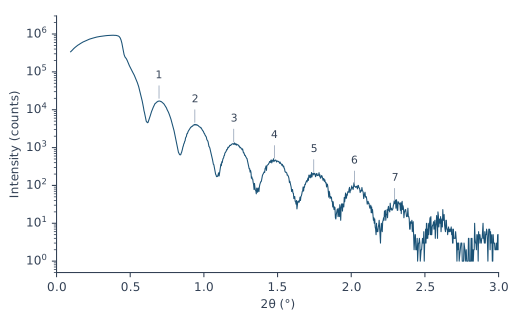
A measured XRR curve of a carbon film on glass on a logarithmic axis, with seven fringe maxima numbered between 2θ of 0.7 and 2.3 degrees — **Figure 5-2:** A measured curve of a single carbon film on glass, with its fringe maxima numbered 1 to 7. Past 2θ = 2.4° the fringes are lost in the counting noise. The intensity is in raw counts on a logarithmic axis. Points with zero counts are left out. Data: curve C1 of the fitting procedure's data deposit, measured with Cu Kα radiation.

Table 5-1: The fringe maxima of Figure 5-2. Each thickness is calculated from one pair of neighboring maxima as H = λ/Δ(2θ), with Δ(2θ) in radians and λ = 1.5406 Å.

Maximum	2θ (°)	Δ(2θ) from the previous (°)	H from the pair (Å)
1	0.696
2	0.939	0.243	363
3	1.202	0.264	334
4	1.478	0.276	320
5	1.746	0.267	331
6	2.022	0.276	320
7	2.295	0.273	323

The spacing is smaller near the edge because of refraction. Inside the film the beam travels at a smaller angle than outside (Chapter 4: A refractive index just below 1). The lag follows the angle inside. So the fringes are evenly spaced in the angle inside the film. Close to the critical angle the two angles differ most. Far above it they are almost equal, and the spacing approaches λ/2H.

The first pair of maxima gives 363 Å. The pairs further out give 320–334 Å. A fit of all seven positions with the refraction included gives 316.8 Å (see the Going Deeper box). A full fit of this curve put 300.5 Å of carbon under a contamination layer 13 Å thick. Together that is 313.5 Å. The fringes measure everything that lies on the substrate, the contamination layer included.

Going Deeper: the fringe positions with refraction

Inside the film, $\theta_t^2 \approx \theta^2 - 2\delta$ , where δ is that of the film. The maxima are evenly spaced in $\theta_t$ , by λ/2H. So the j-th maximum lies at

\theta_j^2 \approx \left(\frac{\lambda}{2H}\right)^2 (j + m_0)^2 + 2\delta

with θ in radians. $m_0$ is an unknown offset, because the first fringe you see need not be the first in the count. A least-squares fit of the seven positions of Table 5-1 for H, $m_0$ and δ gives H = 316.8 Å. The Bragg law with refraction in Chapter 6: The Bragg law with refraction has the same form.

A fringe needs enough points to be seen. With fewer than two points per fringe, the measured points skip across the fringes. The fringe heights can then seem to rise and fall slowly, which the film does not cause. The curve of Figure 5-2 has a step of 0.003° in 2θ, about 90 points per fringe. Data > Assess XRR quality … checks the points per fringe of a measurement. Fringes closer together than the resolution of the instrument are blurred away before they are counted. For them the check judges the step against the resolution instead (Chapter 10: When not to fit).

What density does to the fringes

The depth of the fringes depends on how strongly each boundary reflects. The top surface reflects like the bare film material. The buried interface reflects according to the difference between film and substrate. Well above the critical angle, the reflectivity of a boundary grows with $(\delta_2-\delta_1)^2 + (\beta_2-\beta_1)^2$ . The indices 1 and 2 stand for the two materials. When film and substrate have nearly the same δ and β, the interface hardly reflects. The fringes are then weak.

Carbon on silicon is such a case. At its bulk density of 2.266 g/cm³, carbon has δ = 7.28 × 10⁻⁶. Silicon has 7.61 × 10⁻⁶ (Chapter 4: Table 4-1). At 1.8 g/cm³ the δ of carbon falls in proportion, to 5.78 × 10⁻⁶. The interface then reflects about 25 times more strongly. Figure 5-3 shows the result for a 200 Å film. At bulk density the fringes are faint: each maximum is less than twice its neighboring minimum. At 1.8 g/cm³ the ratio is 4 to 11. A 200 Å molybdenum film on silicon has a ratio of 22 to 36.

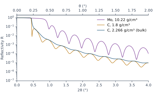
Calculated reflectivity of 200 angstrom films on silicon: molybdenum with deep fringes, carbon at 1.8 grams per cubic centimeter with clear fringes, and carbon at bulk density with faint fringes — **Figure 5-3:** Calculated reflectivity of three 200 Å films on Si at λ = 1.5406 Å, all smooth. Carbon at its bulk density, 2.266 g/cm³, is optically close to silicon. Its fringes are faint. At 1.8 g/cm³ they are clear. The dense Mo film has deep fringes. It keeps a high reflectivity up to its own critical angle, at 2θ ≈ 0.87°. Calculated by X-Ray Calc 3.9.4.1250 with no resolution blur.

A dense film also moves the critical edge. The 200 Å Mo film in Figure 5-3 reflects 74 % of the beam at θ = 0.40° and 40 % at θ = 0.45°. Its edge sits at the critical angle of Mo, 0.434°, well above the 0.224° of the silicon under it.

What roughness does to the fringes

A film has two roughnesses: that of its top surface and that of the interface with the substrate. In X-Ray Calc the σ of a layer is the roughness of its upper interface. So the σ field of the film is the roughness of the top surface. The σ field of the substrate is the roughness of the buried interface.

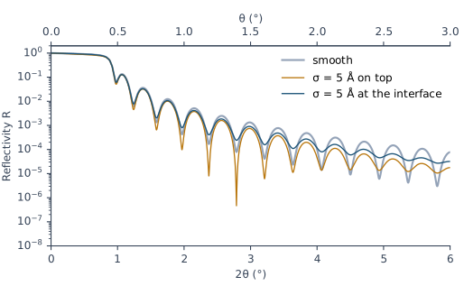
Roughness weakens the reflection of a boundary. It weakens it more at larger angles. The fringes are deepest when the two boundaries reflect equally. When one of them stops reflecting, the fringes fade. Figure 5-4 shows both cases for a 200 Å Mo film on Si:

σ = 5 Å at the interface. The fringes fade steadily with angle. The maximum-to-minimum ratio falls from 16 at θ = 0.53° to 1.7 at θ = 2.78°. The smooth film has 22 and 36 at the same fringes. The mean level of the curve hardly changes.
σ = 5 Å on the top surface. The whole curve falls faster. Between θ = 2° and 2.8° its mean level is half that of the smooth film. The fringes first become deeper, with a ratio of 472 at θ = 1.08°. Then they fade, to 2.5 at θ = 2.79°. The smooth Mo surface reflects more strongly than the Mo/Si interface. A rough top first balances the two reflections. At larger angles it makes the top the weaker one.

Calculated reflectivity of a 200 angstrom molybdenum film on silicon: smooth, with 5 angstrom roughness on top, and with 5 angstrom roughness at the interface — **Figure 5-4:** Calculated reflectivity of a 200 Å Mo film on Si at λ = 1.5406 Å. Gray: both boundaries smooth. Orange: σ = 5 Å on the top surface (the σ of the film). Blue: σ = 5 Å at the film/substrate interface (the σ of the substrate). Roughness at the interface flattens the fringes. Roughness on the top lowers the whole curve. Calculated by X-Ray Calc 3.9.4.1250 with no resolution blur.

Chapter 7: A boundary with a width explains how X-Ray Calc models roughness.

What this means when you fit

The positions of the fringes fix the thickness. For the film of Figure 5-2 they give 316.8 Å, about 1 % above the fitted total. The depth of the fringes depends on the density of the film and on the roughness of both boundaries at the same time. A light film on a substrate of similar δ gives weak fringes. They cannot separate these effects. For such a film the fitting procedure reports the thickness only. It gives σ and ρ as undetermined. Of the film in Figure 5-2 the methods paper says: “The film yields its thickness, and nothing further.”

So set the starting thickness of a film from its fringe spacing, measured far above the edge. Chapter 12: The periodic stack shows where this value goes.

A one-layer model may not reproduce the critical edge or the fringe contrast of a light film. Neither the resolution nor the substrate roughness is the cause, so don’t try to repair it with them. For the carbon film of Figure 5-2, no model reproduced both. Chapter 7: The dirty surface: a contamination layer describes the layer that every surface carries in air. Chapter 21: Fitting the carbon film fits this film and reports it.

Sources

Fitting procedure (Penkov, Peng & Fu 2026), §12.1–12.2: a single film of the light material gives its thickness and nothing else, with σ and ρ reported as undetermined; a one-layer model does not reproduce the critical edge or the fringe contrast of such a film, and neither the resolution nor the substrate roughness is the cause.
Methods paper, Supplementary S4 (si\S4-results-in-full.md): S4.6, the refit of C1 at 300.5 Å under a contamination layer 13 Å thick; S4.7, “No model of the single carbon film C1, by the expert or by any session, reproduced both its critical edge and its fringe contrast. The film yields its thickness, and nothing further.”
The measured curve C1 (record P2-06, a single carbon film on glass) is from the fitting procedure’s data deposit (CC BY 4.0). It is read in place and not copied into the book. Its file records Cu Kα, λ(Kα1) = 1.5405980 Å, and a 2θ step of 0.003°.
Spiller, E. (1994). Soft X-ray Optics. SPIE. The phase gained in a layer, ½qd, with the angle inside the layer from Snell’s law (p. 104, Eq. 7.2); the reflection of one film, r = (r_t + r_b e^(2iφ))/(1 + r_t r_b e^(2iφ)), and its repeated use for a stack (p. 105, Eq. 7.6); the Bragg condition with refraction (p. 106, Eq. 7.7), whose form the chapter applies to the film thickness; the reflectivity of a boundary well above the critical angle, [(δ₂ − δ₁)² + (β₂ − β₁)²]/(4 sin⁴θ) (p. 26, Eq. 3.12); the modulation largest when both boundaries reflect equally, and fading at large angles as the rougher boundary stops reflecting (p. 201); a false slow oscillation from too few sampling points (p. 109, Fig. 7.2 caption). Spiller gives no single-film fringe-spacing formula. The chapter derives Δθ ≈ λ/2H from Eq. 7.2. Spiller writes d for the thickness; the chapter writes H.
X-Ray Calc Help: Data → Assessing a Measurement (the points-per-fringe check: fewer than two points per fringe fails); Charts → Interaction, Cursor Tracking.
The X-Ray Calc 3 source: the Chart Info bar’s X, Y, Rmax and Xmax, which read the active model’s calculated curve inside the zoomed range (XRayCalc3\Views\frame_ChartInfo.dfm, frame_ChartInfo.pas:254–288, 394–403); σ of a layer as the roughness of its upper interface (unit_calc.pas:642, NOTATION).
Calculated for this chapter (2026-09-24, rerun 2026-09-25) with the X-Ray Calc 3.9.4.1250 engine at λ = 1.5406 Å, with no resolution blur and s-polarization: the 200 Å films of Figures 5-3 and 5-4. scripts/figures/ch5_engine_data.py runs the calculations and keeps the curves in figures-src/ch5/. scripts/figures/fig_5_figures.py draws Figures 5-2 to 5-4. It also finds the C1 maxima of Table 5-1, fits them with refraction (316.8 Å), and computes every contrast ratio and mean level quoted in the text. The δ of carbon at 1.8 g/cm³ and the factor of about 25 are computed on the page from the Henke values of Chapter 4.

Cross-references: Chapter 1: Figure 1-2; Chapter 4: The critical angle and the plateau; Chapter 6: A stack that repeats; Chapter 7: The dirty surface: a contamination layer; Chapter 8; Chapter 10; Chapter 12; Chapter 21: Fitting the carbon film; Appendix D: Glossary.